We have found a linear model for our data, however, we still need to find the error in our model. We know there is error because some of the data points are not on the line.
The error we care about is called the "residual." It is the vertical distance between each point and the line. If a point is above the line, it will have a positive residual. If it is below, the residual will be negative. If it is on the line, the residual will be negative.
The residual is a change in y-value. So, let us look at a specific example before going on.
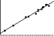
The plot below shows the three points (1,1), (2,4), and (3,3) along with the linear regression line that corresponds to the three points y1 = x + 2/3.
Since there are three data points, we need to find three residuals. Let's start with the point (1,1). How far below the line is (1,1)? Well, if we plug x=1 into y1, we find that y1(1) = 5/3. Since the y-value of point is y = 1 and the y-value of the line is at y = 5/3, the residual = 1 - 5/3 = -2/3. Notice that the residual is negative. This is because the line is above the point.
Moving on to the second point, (2,4) we find that y1(2) = 8/3. But the point has a y-value of y = 4 and so the residual = 4 - 8/3 = 4/3. The residual is positive since the point is above the line.
Finally, the residual of the third point is residual = 11/3 - 3 = -2/3 as with the third point.
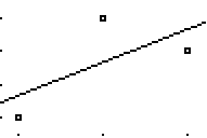
The plot of these residuals is:
Notice that the residual (or error) is along the vertical axis. So, the residual when x = 2 is y = 4/3. Also note that the scale is different than that above. (More on this later.)
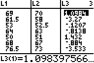
To generalize from the example, to calculate the residual, we take the y-values of the points (which are found in L2) and subtract the y-values on the line. To find the y-values on the line, we plug the x-values (found in L1) into the function Y1. So, we get the formula:
Residual = L2 - Y1(L1).
To calculate this, go the lists and move the cursor to L3:
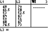
L3 is going to be our residuals, so type in "L2 - Y1(L1)." Then press ENTER.
Note: To get Y1, type VARS, Y-VARS, Function, Y1. For more detailed directions on getting Y1, click here.
Your L3 should now look like that below:
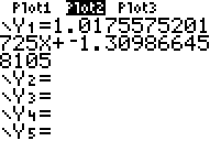
To plot the residuals, go to the Y= and turn Plot1 off and Plot2 on. Also, turn Y1 off since we don't need to see the line when we are plotting the residuals.
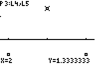
Now press ZOOM and then 9 to choose ZoomStat (more). This will give you the residual plot below:
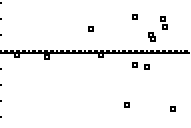
The horizontal axis measures the person's height and the vertical axis measures the residual. In this case, the residual is the difference between the arm span predicted by the model and the person's real life arm span.
Note 1: The residuals are very random looking. This is good since it tells us that we were right to choose a linear model. If there was a pattern in the residuals, we would have to go to plan b. (Plan b is not a part of this example;-).
Note 2: The data is a skewed to the right - that is, there are only a couple of points on the left. This is because I only measure a couple of babies, but measured a bunch of adults.
Perhaps you are thinking that the residuals look really big, if so, consider the following two screen shots:
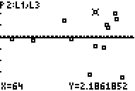
Notice that the error in the approximation of the marked point (top center) is only 2.18 inches.
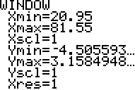
This window shows that the residuals measured along the y-axis are always between -4.5 and +3.15. This means that the error at most a couple of inches.
Now that we have the residuals, we can find an "average error." This will be used to find error bounds. These error bounds will be used when you use the model to approximate a person's arm span.
last modified September 05, 2007