back

Error Bounds.

Navigating the Process.

1. Clearing Your Lists.
2. Clearing your Y=.
3. Entering Your Data.
4. Setting up STAT PLOT.
5. To Select Which STAT PLOT to Graph.
6. Plotting L1 vs. L2.
7. Linear Regression.
8. Residuals.
9. ***Error Bounds.

Contents.

1. Overview.
2. Sample Standard Deviation.
3. Example.
4. Error Bounds.
5. Do It On Yourself.
6. Conclusion.

Overview.

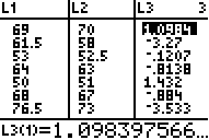
In looking at our residuals, we notice that none of the residuals are exactly zero.  (See L3 below).  However, we want to use our model to predict someone's arm-span given their height. 

Sample Standard Deviation.

We need to determine what kind of error we can expect in our approximation.  To do this, we will find some measure of average residual.  For reasons I won't go into here, we will use the standard deviation of the residuals - specifically the sample standard deviation.

To find the sample standard deviation, press STAT.  Right arrow over to CALC.  Then choose option 1, 1-Var Stats.  This will give a home screen like:

Type L3 since this is the list that contains the residuals.  Then press ENTER.  You will get the results:

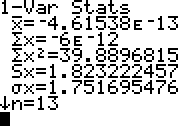
The sample standard deviation is Sx = 1.823222457.

Write Sx down on a piece of paper.

In statistics (like Math 210), we learn that 95% of a normally distributed population (think data set) is within 2 standard deviations of the average.  In our case, two standard deviations are about 2*Sx = 3.6464 inches. 

So, multiply Sx by 2 and write down this result (2*Sx).

Example.

So, for example, if Dusty is 6' 1" in height, then he is 73" tall.  We approximate his height by calculating Y1(73):

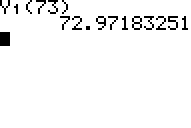  (Get Y1 by typing VARS, Y-VARS, Function, Y1).

So, we approximate Dusty's arm span at 72.9718 inches (just less than 6' 1").  However, this doesn't take into account the error in the approximation.

If we assume our data was normally distributed, we can have 95% certainty that Dusty's actual arm span is 72.9718 +/- 3.6464.  That is, there is a 95% chance that Dusty's actual arm span is between 69.3254" and 76.6182".

Dusty's actual arm span was 75" which is definitely within our bounds.

Error Bounds.

We want to include our bounds with our model (model is Y1(x)).  So, including the bounds, our model is:

Y1 = 1.0175575201x - 1.30986645 +/- 3.646444914.

To plot this, we plot our model, the upper bound (+), and the lower bound (-).  That is, we plot:

1.) Y1(x).
2.) Y1(x) + 3.646444914
3.) Y1(x) - 3.646444914.  

My Y= looks like:

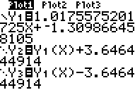
Pressing GRAPH reveals the plot below.  Notice that I highlighted the point representing Dusty (upper right).

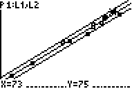
Notice that every single point looks like it is between the error bounds.

Problem.

Measure your height and then use the model to predict your own arm span.  Using the error bounds, what is the range where your arm span should lie?  Measure your arm span and check to see if the model works.

Conclusion.

That is all there is to linear data analysis.  All you have to do now is to do it - and then interpret your results;-)

Navigating the Process.

1. Clearing Your Lists.
2. Clearing your Y=.
3. Entering Your Data.
4. Setting up STAT PLOT.
5. To Select Which STAT PLOT to Graph.
6. Plotting L1 vs. L2.
7. Linear Regression.
8. Residuals.
9. ***Error Bounds.

  last modified December 16, 2010