How to build efficient systems of
spreadsheets to save time, get promoted and have extra time for vacation
An Excel book that takes you from the beginning
theories of how to construct efficient systems of spreadsheets towards the
Beautiful Excel infinity at the other end
By Michael
“Excel Is Fun!” Girvin
Warning: because this book is free, I could not afford an
editor. So you will have to put up with the occasional spelling/grammatical
error. If you find any kind of error, please e-mail me at mgirvin@highline.edu.
Dedication:
This book is dedicated to Dennis “Big D” Ho, my step-son,
because he loves books so much!
This book is also dedicated to Isaac “Big I” Girvin, my son,
because he is so inquisitive!
Table of
Contents
Introduction. 4
What
Is Excel?. 5
Rows,
Columns, Cells, Range Of Cells. 7
Worksheet,
Sheet Tab, Workbook. 8
Save
As is different than Save. 10
There
are no more Menus or Toolbars in Excel 2007. We now have “Ribbons”, the “Orb”
and the “QAT” toolbar. 11
Ribbons. 13
Quick
Access Toolbar (QAT) 21
Scroll
Bars and Selecting Cells. 24
Keyboard
Shortcuts and the Alt Key. 27
Two
Magic Characters In Excel 32
Math. 38
Formulas. 42
Functions. 47
Cell
References. 57
Assumption
Tables/Sheets. 72
Cell
Formatting. 82
Charts. 105
Page
Setup. 115
Analyze
Data: Sort, Filter, Subtotals, PivotTables. 121
IF
function. 135
Conclusion: 140
Excel is Fun! Why? Because your
efficient use of Excel can turn a three hour payroll calculating chore or a
five hour reporting task into a five minute breeze. Efficient use of Excel will
save a lot of time. That time adds up to extra time for your more enjoyable
endeavors in life such as vacations! In addition, your bosses and employees
will notice that you are efficient and can produce professional looking reports
that impress. This of course leads to promotion more quickly. Still, further,
your knowledgeable and efficient use of Excel can land you a job during an
interview. Employers are like dry sponges ready to soak up any job candidate
that can make their entity more efficient with Excel skills! Save time?, get
promoted?, get the job?, and have more time for vacation? – That sounds like a
great skill to have!
In the working world, almost
everyone is required to use Excel. Amongst the people who are required to use
it, very few know how to use it well; and even amongst the people who know it
well, very few of those people know how to use it efficiently to the point
where grace and beauty can be seen in a simple spreadsheet!
This book will take you from the
very beginning basics of Excel and then straight into a simple set of
efficiency rules that will lead you towards Excel excellence.
You use Word to create letters,
flyers, books and mail merges. You use PowerPoint to create visual, audio and
text presentations. You use Google to research a topic and find the local pizza
restaurant. You use Excel to make Calculations,
Analyze Data and Create Charts. Although databases (such
as Access) are the proper place to store data and create routine calculating
queries, many people around the planet earth use Excel to complete these tasks.
Excel’s row and column format and ready ability to store data and make
calculations make it easy to use when compared to a database program. However,
Excel’s essential beauty is that you can make calculations and analyze/manipulate
data quickly and easily “on the fly!” This easy to use, planet-earth “default”
program must be learned if you want to succeed in today’s working world.
Open up the Excel file named “Excel
2007 Is Fun!.xlsm” and with your mouse, click on the “What is Excel” sheet tab.
Here is an example of how Excel can make payroll Calculations quickly and with fewer
errors than doing it by hand (Figure 1)
(Your sheet will not appear as large as the one in Figure 1):

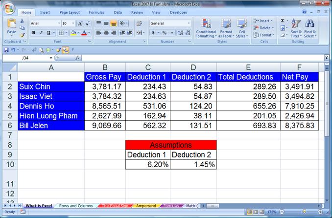
Figure 1
Here is an example of how Excel
can Analyze Data (sorting by time)
quickly and with fewer errors than doing it by hand (Figure 2 and Figure 3):
With your mouse, click on the
“Rows and Columns” sheet tab.

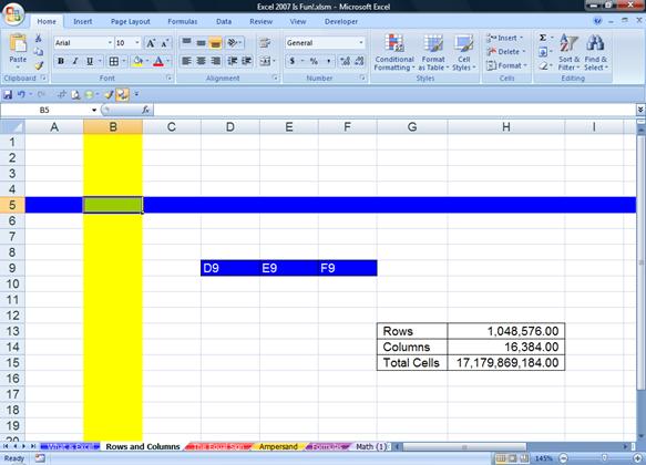
Figure 4
Rows are horizontal and are
represented by numbers. In our example (Figure 4)
the color blue has been added to show row 5.
Columns are vertical and
represented by letters. In our example (Figure 4)
the color yellow has been added to show Column B.
A cell is an intersection of a row
and a column. In our example the color green has been added to show cell B5. In
our example column B and row 5 can be detected because the column and row
headers are highlighted in a light-orange color (Figure 4) (color may vary by computer). In addition, you can see that the
name box shows that cell B5 is selected (Figure 4
and Figure 5).
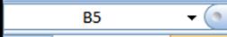
Figure 5
B5 is the name of this cell. It
can be thought of as the address for this cell. It is like the intersection of
two streets. If we wanted to hang out at the corner of Column B Street and Row 5 Street, we
would be hanging out at the cell address B5.
Later when we make calculations in Excel (making formulas),
B5 will be called a cell reference.
A range of cells is two or more
cells that are adjacent. For example you can see three blue cells D9, E9, and
F9. This range would properly be expressed as D9:F9, where the colon means from
cell D9 all the way to cell F9.
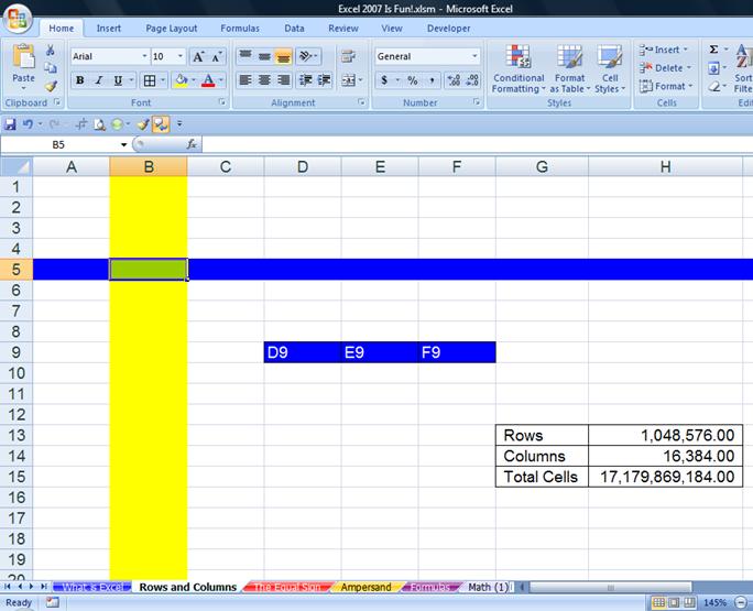
Figure 6
A worksheet is all the cells (1,048,576
rows, 16,384 columns worth of cells). A worksheet is commonly referred to as
“sheet.”
The sheet tab is the name of the
sheet. By default they are listed as Sheet1, Sheet2. In our example (Figure 6), the sheet we are viewing is named “Rows and
Columns.” You can see other worksheets that have been given names in our
example. Can you see what they are?
Naming your sheets helps you to
keep track of things in a methodical way. Navigating through a workbook,
understanding formulas and creating headers/footers is greatly enhanced when
you name sheets. To name your sheet, double-click the sheet tab (this highlights
the sheet tab name) and type a logical name that describes the purpose of the
sheet. You can also, right-click a sheet tab and point to Rename in order to
give the sheet a new name.
A workbook
is all the sheets (over 8000 worksheets possible – limited my computer’s memory).
To name a new workbook that has not been saved or named, use Save As (Keyboard Shortcut = F12).


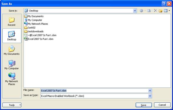
Figure 7
Figure 7 shows the Save As dialog box:
Save in = Where do you want to
save it?
File name = What do you want to
call it?
Save as type = What type of file
is it? (.xlsm? or .xlsx or .xls or .htm? or .xltm or .xlt?)
See notes on next page about the
new Excel 2007 “Save as types”.
Some of the Excel 2007 “Save as
type” or “extension type” or “file format”:
1.
xlsm
i.
2007 workbook that allows Macros (Macros = custom code
that you can put in workbook (VBA))
ii.
This file format is called XML (Extensible Markup
Language). XML is efficient because:
1.
Most any program can read it
2.
It is less corruptible
i.
Lose a few lines in BIFF and you can lose the whole
file, lose a few lines in XML and you can easily recover the file
iii.
This new file format is different than XML in 2003 (2003
XML did not support VBA, Charts, and other embedded images), it now supports
all Excel elements.
iv.
These files are actually zipped files!!!!
i.
Saves space
2.
xlsx
i.
This is the same as the description for .xlsm except that
does not allow Macros (Macros = custom code that you can put in workbook(VBA))
3.
.xls
i.
1997 – 2003 file format
1.
Use this if you are going to let other people
use your file that do not have Excel 2007
4.
.htm
i.
Saves worksheet or workbook as html (web site)
5.
.xltm
i.
2007 Excel Template that allows Macros
1.
Templates automatically save to the Microsoft
Template folder so that your template will show up in the Templates window
6.
.xlt
i.
1997 – 2003 file format for Templates
7.
.xlsb
i.
This file type is called BIFF (Binary Interchange File
Format)
1.
BIFF5 (Excel 95)
1.
BIFF8 (Excel 97-2003)
2.
BIFF12 è.xlsb
i.
BIFF cannot be read by many applications
ii.
But it saves and loads more quickly than XML
Once you have saved your workbook for the first time,
subsequent saves will replace the stored file with the most recent changes. Save
As gives you the power to: 1) Save the file to a new location 2) save file with
a new name 3) change the file type. In this way the Save As dialog box is very
powerful.
The menus and toolbars from
earlier versions of Excel are gone. In their place are “Ribbons” and the “Quick
Access Toolbar” (QAT). The Ribbons contain icons and words that let you click
on a particular icon to take a particular action such as changing the font size
or changing the number of decimals showing for a number. The icons and words
are grouped into categories to help the user find similar items. These
categories are called “Groups”. There are 26 total different Ribbons. You can
only view one Ribbon at a time. The “Orb” or “Office Button” (located in the
upper left corner of the screen, to the left of the Home Ribbon and slightly on
top of the title bar) shows a “Microsoft Office” icon inside a glowing circle.
If you click on the Orb a drop-down menu appears (similar to the old File menu)
that has icons and words that let you click on a particular icon to take a
particular action such as Save As or Excel Options. The QAT contains the icons
for save, undo and redo by default and then any other additional icons that you
add yourself. There is only one QAT. The QAT is always visible and available
for use, either above the Ribbons or below the Ribbons depending on where you
place it.
The Ribbons change appearance depending on the size of your
screen and/or your computers screen resolution (screen resolution can be
changed in Display Properties). The QAT changes appearance depending on how you
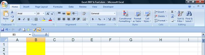
customize it. Figure 8 shows the Home
Ribbon on a large screen (or high screen resolution) and with a QAT that has five
additional icons beyond the three default icons. Figure 9 shows the Home Ribbon on a small screen (or low screen
resolution) and with a QAT that has 23 additional icons beyond the three
default icons.


Quick Access Toolbar (QAT)
|
|
Figure 8


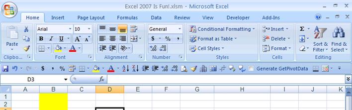
Figure 9
Figure 10 Shows the
Orb drop-down menu and the Excel Options button. You can see the icons and
words such as Save As, the list of recent Documents that have been used and are
accessible here to re-open, and the Excel Options button in the lower right
corner.
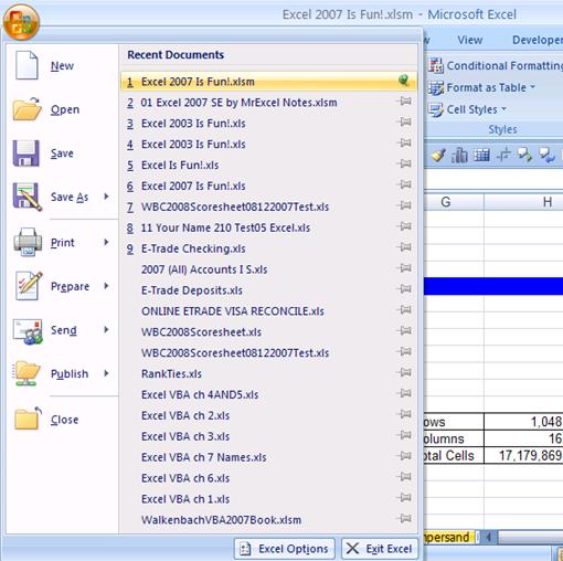
Figure 10: Orb drop-down menu and Excel
Options button that appear after you click the Orb.
Now we would like to talk about the Ribbons in more detail.
Each Ribbon has a tab that sticks out above the Ribbon and
contains the name of the Ribbon. There are seven standard Ribbons (Home,
Insert, Page Layout, Formulas, Data, Review) and 18 additional Ribbons. Some of
the addition Ribbons you can add in the Excel Options Area and some of the additional
Ribbons are “Context-Sensitive Ribbons” (also known as “Contextual Ribbons”)
that show up depending on where the cursor is located (for example, if a chart
is selected, the context sensitive Ribbons for charts appear). To move between
the visible Ribbons you can click on any tab name to access that particular
Ribbon. If you want to temporarily hide the Ribbons because of space
requirements, use the keyboard Shortcut Ctrl + F1 (This is a toggle that will
successively hide and unhide the Ribbons). The seven standard Ribbons, one
additional Ribbon added in Excel Options and one context sensitive Ribbon are
shown below in figures: Figure 11 to Figure
20.
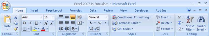
Figure 11: Home Ribbon: Contains items such as
Copy, Paste, stylistic (Font/Color) formatting, Number Formatting, Conditional
Formatting, Insert Row/Column, Insert Function, Clear All, Clear Format,
Sorting, Find, Replace, Select, Go To, Go To Special, and more….
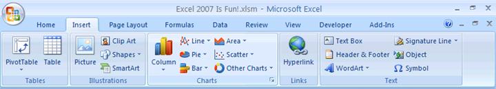
Figure 12: Insert Ribbon: Insert items such
as: PivotTable, Table, Pictures, Clip Art, Shapes, Charts, Hyperlinks, Text Box,
Header and Footer, Word Art, Object, or Symbol.
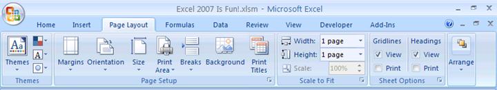
Figure 13: Page Layout Ribbon: Add
Themes (coordinated Color, Font, Effects), various page layout for printing.
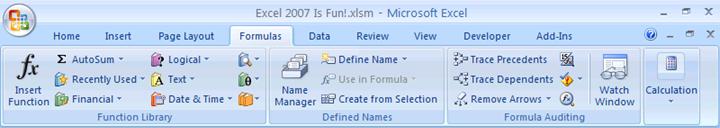
Figure 14: Formulas Ribbon: Contains
items such as Insert Functions, Insert Functions Categories, items associated
with Names, items associated with Formula Auditing, and Calculation.
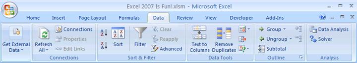
Figure 15: Data Ribbon: Get External
Data, Refresh (External Data or PivotTable), Sorting and Filtering, Text to
Columns, Data Validation, Consolidate, Scenario Manager, Goal Seek, Data Table,
Grouping, Subtotals, and the Add-ins Data Analysis (statistics) and Solver (linear
algebra) if you add them using Add-ins in the Excel Options area.
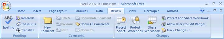
Figure 16: Review Ribbon: Contains
items such as Spell Check, Comments, Protect Worksheet or Workbook, Share
Workbook and Track Changes.
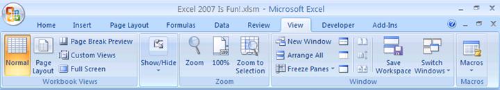
Figure 17: View Ribbon: Contains items
such as Normal view, Page Layout view, Page Break Preview view, Show/Hide
Formula Bar, Show/Hide Gridlines, Zoom view, New Window (opens a second view of
the same Workbook), Arranges All (arranges all open Workbooks), Freeze Panes (always
show a certain part of the Worksheet), Hide Window (which means hide Workbook),
Unhide Window (which means unhide Workbook), Save Workspace, Macros (Macro means
Excel computer code that you can write Excel).
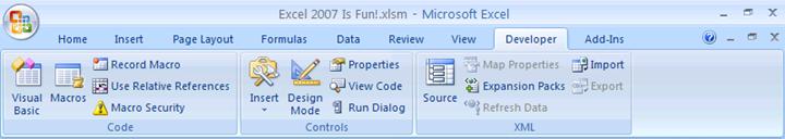
Figure 18: Developer Ribbon that was
added in the Excel Options area.
To add the Developer Ribbon you would use the keyboard
shortcut to get to Excel Options as follows: Alt + F + I (Tap the Alt key, then
tap the “F” key, then tap the “I” key). Excel Options is also accessible by
clicking on the Orb and then click on the Excel Options button. After you open
the Excel Options dialog box, you would check the “Show Developer tab in the
Ribbon” checkbox and then click the OK button and the lower right corner. See Figure
19:


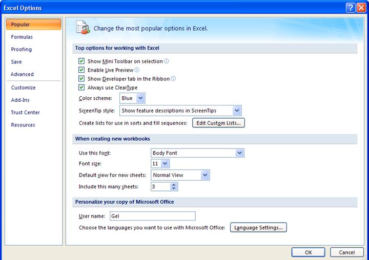
Figure 19: Excel Options
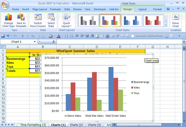
Figure 20: Because a Chart is selected, the Title
Bar shows “Chart Tools” and there are three context sensitive chart Ribbons
after the last “always-available” Ribbon. The three Chart Ribbons are: Design,
Layout, Format.
As seen in Figure 21
and Figure 22, some of the elements of
the Ribbons are:
- Tabs (Page Layout)
- Groups (Page Setup
Group)
- Icons (Orientation)
- Drop-down arrows
(Orientation: Portrait or Landscape)
- Check Boxes (Toggle to
view or not view Excel Gridlines)
- Dialog Launchers (Small
grey boxes with diagonal arrows that, when clicked, launch the 1997-2003-type
dialog boxes – you can see the Page Setup Dialog launcher on the right-side
of the Page Setup Group Label)


 “See More Selections” Arrows (Figure 22 shows More Chart Styles)


7) “See More Selections” Arrow
|
|
 Figure 21
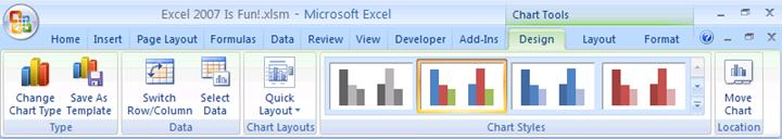
Figure 22
The Ribbon elements can be seen in further detail in the
figures .
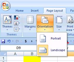
Figure 23: If you click on the
Orientation drop-down arrows you can see the two options for printing your
worksheet: Portrait or Landscape. The shaded box means that the current
selection is Landscape. If you clicked on Portrait, you would change the printing
orientation to Portrait.

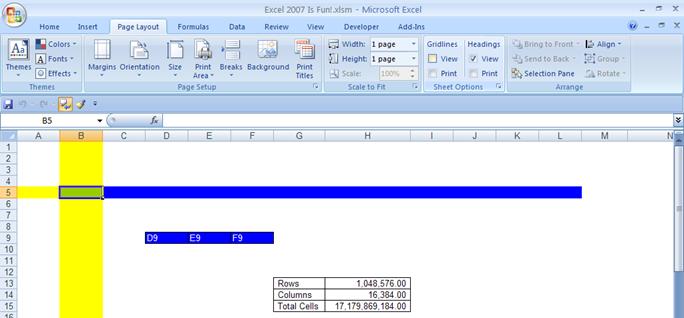
Figure 24: The check box for View
Gridlines in the Sheet Options Group has been unchecked. The result is that the
default Excel Gridlines cannot be seen on the screen and they will not be
printed. Compare this to Figure 6. In Figure
6 you can see the Gridlines. The Check Boxes
are “Toggles” that will alternate between viewing the Excel Gridlines and not
viewing the Excel Gridlines. Notice that the black lines around the Row and
Column count are still viewable. This is because these lines were added using
the borders button in the Font Group on the Home Ribbon.
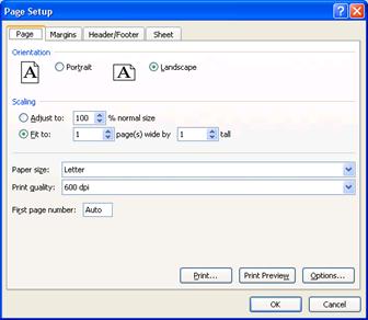
Figure 25: If you click the Page Setup
Dialog Launcher on the right-side of the Page Setup Group Label this dialog box
will show up. This is the Excel 1997-2003 Page Setup dialog box.
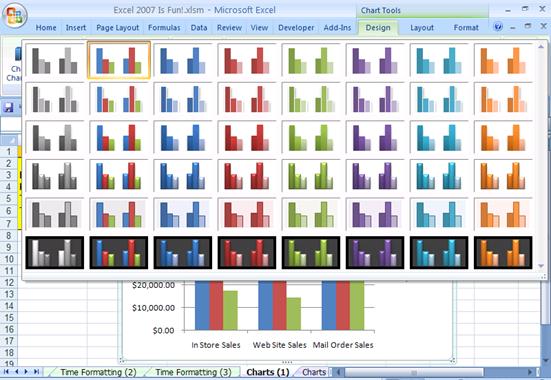
Figure 26: If you click the “See More
Selections” Arrow in the Chart Styles Group in the Chart Tools Design Ribbon
you will see more selections for Chart Design.
The last important trick regarding the Ribbons is that you
can hide them. This is convenient because they take up a lot of room on the
screen. The keyboard shortcut for toggling the Ribbons on and off is Ctrl + F1
(Hold Ctrl and then tap the F1 key (the F1 key is in the top row of keys on the
keyboard and all the way to the left, but to the right of the Esc key)). See
figures Figure 27 and Figure 28 for examples of the Ribbons toggled off and
toggled on.
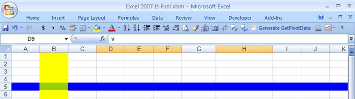
Figure 27: Ctrl + F1 hides the Ribbons, but
the QAT is still visible!
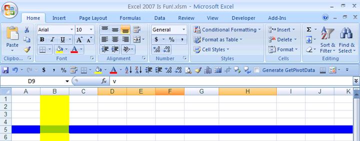
Figure 28: Ctrl + F1 a second time, toggles
the Ribbon on again.
Now we would like to talk about the Quick Access Toolbar (QAT)
in more detail.
No matter what Ribbon you have showing, or whether or not
the Ribbons are toggled on or off, the QAT is always visible and available for
use! This is great because sometimes it is quicker to click on the QAT than it
is to click on the Ribbon and then click on the icon you want. Not only that,
but there are actions, dialog boxes and Task Panes from Excel 1997-2003 that
are not anywhere in the Ribbons! So if you have a particular action that you
used to do in earlier versions of Excel and it is not in the Ribbons, you can
add it to the QAT. Also, you can easily show your QAT above or below the
Ribbon. First let’s see two great ways to add icon buttons to the QAT.
The first way to add icon buttons to the QAT is to find an
icon or an item from a drop-down arrow list in the Ribbons, and then
right-click that item. If the right-click drop-down menu says “Add to Quick
Access Toolbar”, then you are allowed to add that icon to the QAT. If you do
not see “Add to Quick Access Toolbar”, then that item is not available to be
added to the QAT (Some items are not available). In Figure 29 I have right-clicked the Fill icon (it is
the picture of a tipping paint bucket – it is the icon button that fills the
cell with color) and you can see the right-click drop-down menu. After I click
on the “Add to Quick Access Toolbar”, the icon button will automatically be
added to the QAT (Figure 30).
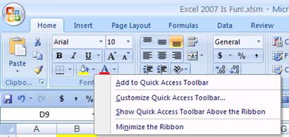
Figure 29: Right-click a Ribbon icon to add it
to the QAT.
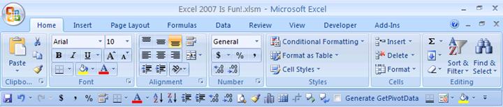
Figure 30: The Fill icon has been added to the
end of the QAT.
The second way to add icon
buttons to the QAT is to go to the Customize section in the Excel Options area.
This is the best method because you can see a list with all the icon buttons
that can be added. In the Figures Figure 31
to Figure 34 the process of adding icon
buttons from the Customize section in the Excel Options area is illustrated.
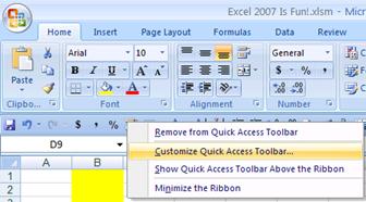
Figure 31: Right-click the QAT and click on
the “Customize Quick Access Toolbar…” item in the drop-down menu.
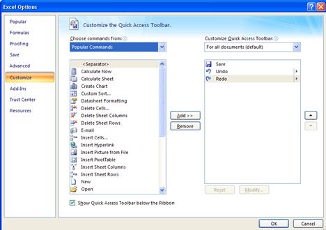
Figure 32: By right-clicking the QAT
and click on the “Customize Quick Access Toolbar…” item in the drop-down menu,
you will automatically go to the Customize section in the Excel Options area.
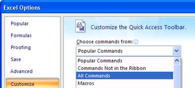
Figure 33: Click on “All Commands” from
the “Choose commands from” drop-down list
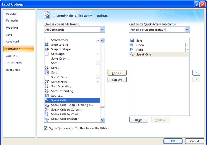


4) Icon will appear on the right
|
|


 Figure 34: Use the Scroll Bar to find the icon
that you want, click on the icon, and then click the add button. The Icon will
appear on the right. When you have added all the buttons that you want, click
the OK button.
Figure 34: Use the Scroll Bar to find the icon
that you want, click on the icon, and then click the add button. The Icon will
appear on the right. When you have added all the buttons that you want, click
the OK button.
The last trick we want to see regarding the QAT is how to
move it above or below the Ribbons. This is easily done. Simply right-click the
QAT and look in the drop-down menu for the command you would like.
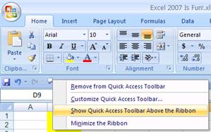
Figure 35: If the QAT is below the
Ribbon and you want to move it above.
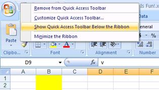
Figure 36: If the QAT is above the
Ribbon and you want to move it below.
In Excel there are Horizontal and Vertical Scroll Bars that
let you move the worksheet so that you can see rows, columns and cells that are
not in view. In addition, for the Horizontal Scroll Bar, you can change the
size of it by clicking on the front edge of the Horizontal Scroll Bar and
dragging. In Figure 37 you can see that I
have labeled the Scroll Bars as Vertical Scroll Bar and Horizontal Scroll Bar,
but technically the whole thing is called the Scroll Bar, the part that you
click on with your mouse and drag is called a “Scroll Box”, and the arrows
(that allow you to move only one row or column at a time) are called “Scroll
Arrows.” Nevertheless, I will refer to the “Scroll Box” as the “Scroll Bar”
because is common language that is the custom.

Technically, this is a Scroll Box, but I will refer to
it as the “Scroll Bar”
|
|


Front edge of the Horizontal Scroll Bar
|
|


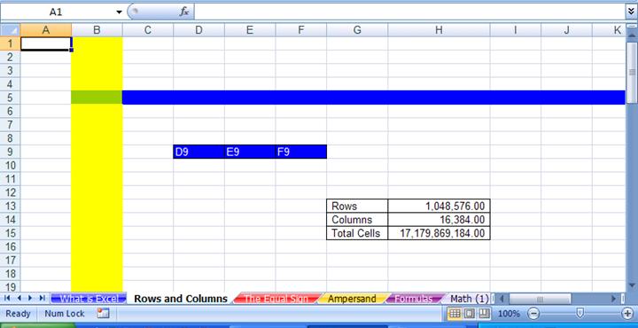
Figure 37
To see how the Scroll Bars work, click on the Vertical
Scroll Bar and drag it down until you can see Row 26. Notice how the first row
now visible is Row 8 (Figure 38):


Small gap means that there are more rows above that are
not visible
|
|

First row now visible is Row 8
|
|
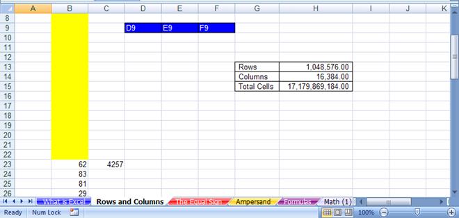
Figure 38
Now use the Horizontal Scroll Bar to move the sheet back so
that you can see Row 1 again (Figure 39):
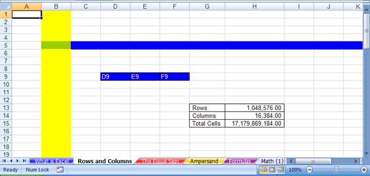
Figure 39
To change the size of the Horizontal Scroll Bar so that the
Horizontal Scroll Bar begins after the Sheet Tab named “The Equal Sign”, click
and drag front edge of the Horizontal Scroll Bar (Figure 40):

Figure 40
Now move it back (Figure 41):

Figure 41
Try moving the sheet with the Horizontal Scroll Bar, and
then move it back.
Next, we want to talk about selecting cells.
Although many of us know how to select something and click
something with your mouse, we will discuss it here so that we are all on the
same page. When you move your mouse in Excel the cursor on the screen moves. However,
the cursor changes depending on what item or element your mouse is hovering
over. To see how this works, make sure you are located on the sheet tab “Rows
and Columns” and then move your mouse over the cell A1 without clicking in cell
A1. You will see a thick-white-cross cursor with a black outline and a black
shadow. Now click in cell A1 and type the number 1. Now when you hover over
cell A1 without clicking in the cell, your cursor is shaped like a thin capital
letter I. Now hit the Enter key and you will see this (Figure 42):
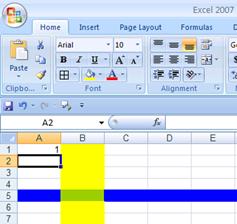
Figure 42
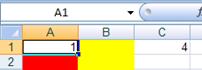
Now take your mouse and move the thick-white-cross cursor
over cell A2, click, hold the click, drag the thick-white-cross cursor to cell
A6, and then let go of your cursor. In Figure 43
you can see that you just have selected the range of cells A2:A6.
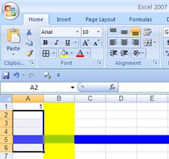
Figure 43
Next, in order to add some color to the selected range,
click the down-arrow next to the Fill icon on the Home Ribbon and select the
color red as seen in Figure 44
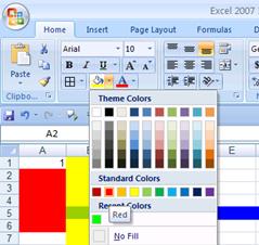
Figure 44
That is how to select cells with the mouse and cursor.
However, there are sometimes when using the mouse to select cells is not
efficient. In our next section, we will see how to use the keyboard to select
cells and how to do many other tasks.
Now we are about to learn the best trick in all of Excel!
Yes, this is the one trick that will guarantee you extra vacation time and instant
success in the eyes of your bosses and co-workers. The one trick is… well it’s
not just one trick, it is many. Are you ready for this?
The best trick in Excel is:
Learn keyboard short cuts!!!!
Keyboard shortcuts are the best way to save time and become
efficient. Let’s look at a few examples here, and then throughout the book, we
will see many more keyboard shortcuts
To see these keyboard shortcuts, make sure you are located
on the sheet tab “Rows and Columns”. Click in the cell C1, type the number 4,
and then hold the Ctrl key and tap Enter. The result is that you have entered
the number 4 in cell C1 and kept your cursor in cell C1 as seen in Figure 45:
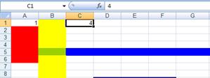
Figure 45
With cell C1 still selected, Hold the Ctrl key and Tap the
‘C” key (this is the keyboard shortcut for copy). After you copy cell C1, you
will see a moving dotted line around the copied cell. Next, to move three cells
to the right and Paste your copied item, Tap the Tab key three times and then
hold Ctrl and tap the “V” key (this is the keyboard shortcut for paste).See Figure
46:
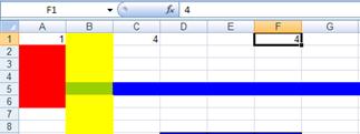
Figure 46
The other benefit to the keyboard shortcuts for Copy and
Paste (besides that they are faster than going up to the Home Ribbon) is that
they work in almost all programs and web sites in the world!
The best example of how keyboard shortcuts can save time is
to show you how to use it when adding. Now we haven’t learned how to make
formulas or use functions yet, but I am going to show you this next keyboard
shortcut for add many numbers in a formula that uses the SUM function before we
even learn about formulas and functions. Why? Because this trick is sooooo much
faster than using a mouse, that it illustrates the beauty of keyboard shortcuts
better than any other trick. Ready? OK. Click in cell B1 (Figure 47):
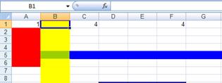
Figure 47
Then hold Ctrl and tap the drown arrow (the arrow keys are
on the right side of your keyboard. Ctrl + down-arrow jumps you to the next
section of data (it skips all the blanks and jumps to the first cell that has a
character). See Figure 48 on the next
page:

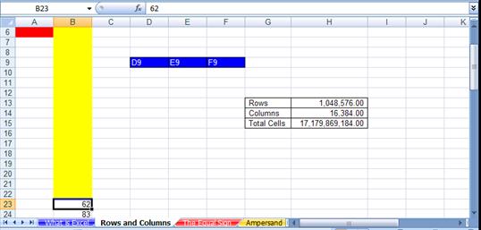
Figure 48: Ctrl + down arrow jumps to the next
section with data, and it also moves the scroll bar so that row 6 is the first row
that we can see.
This also moved the scroll bar so that row 6 is the first
row that we can see (rows 1 to 5 are still in the worksheet, they are just not
visible. Next, hit the Tab key so that your cursor is in cell C23 (Figure 49):
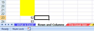
Figure 49
Next, to automatically add a formula that will add, Hold the Alt key and
tap the “=” sign (“=” sign key is to the left of the Backspace key). Atl + = is
the keyboard shortcut for the Auto Sum Function Formula. You should see this (Figure
50):
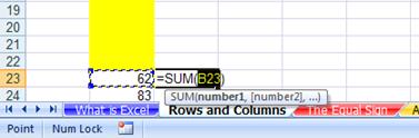
Figure 50
Next, hold the Ctrl key and hold the Shift key at the same
time, and then tap the down arrow key (this selects the entire range of numbers
below cell B23). You should see this (Figure 51):
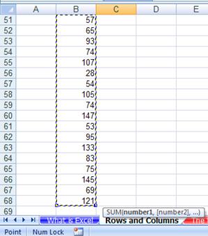
Figure 51
Next tap the Enter key, and the up arrow key five times (the
Enter is to put the formula in the cell and the up arrow keys are to move the
screen down so you can see what you did). You should see this (Figure 52):
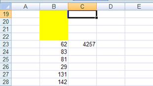
Figure 52
Next, hit the down arrow key four times to select cell C23.
In the formula bar you can see the amazing formula that you created with the
keyboard shortcut Alt + =, then Ctrl + Shift + down-arrow, then Enter. The
formula bar shows that you used the SUM function and selected 46 rows of
numbers without ever using your mouse!!! You should see this (Figure 53):

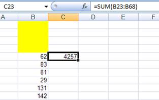
Figure 53
Next, to navigate quickly to cell A1, hold Ctrl and tap the
“Home” key (the Home key is to the right of the Backspace key and above the
arrow keys). Your cursor should be in cell A1 (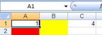 Figure
54):
Figure
54):
 Figure
54
Figure
54
Here are some common keyboard shortcuts:
1. Copy = Ctrl + C
2. Cut = Ctrl + X
3. Paste = Ctrl + V
4. Save = Ctrl + S
5. Spell Check = F7
6. Undo = Ctrl + Z.
7. Redo = Ctrl + Y
8. Go to cell A1 = Ctrl + Home
9. Add bold to cell content = Ctrl + B
10. Add Underline to cell content = Ctrl + U
11. Add Italic to cell content = Ctrl + I
12. Select two cells and everything in-between = Click on
first cell, hold Shift, Click on last cell
13. Select cell ranges that are not next to each other =
click on cell or range of cells, Hold Ctrl, click on any number of other cells
or range of cells
14. Ctrl + arrow key = move to end of range of data, or to
beginning of next range of data
Next we want to look at the keyboard shorts using the Alt
key. The Alt key is a special keyboard shortcut key because when you tap the
Alt key, all the elements in the Ribbon and QAT show little messages called
“Screen tips” or “ToolTips”. To illustrate, tap the Alt key once and you should
see this (Figure 55):

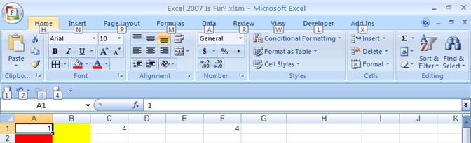
Figure 55: After you tap the Alt key, the
Ribbon Tabs show tool tips and the QAT shows tool tips after the first Alt tap.
If you tap the Alt key once the Ribbon Tabs show tool tips
and the QAT shows tool tips, but none of the other elements of the Ribbon show
screen tips. However, if you tap one of the keys for the letters or numbers
that you see in the tool tips that activates the next level of tool tips. For
example if you hit the “H” key after you taped the Alt key, you would see this
(Figure 56):

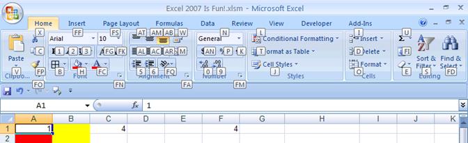
Figure 56: After you hit Alt + H, you can see
the next level of tool tips for the Home Ribbon.
After you hit Alt + H, you can see the next level of tool
tips for the Home Ribbon. If you then tap the 0 key (zero key), you would have
increased the decimals showing by one position. Thus, the keyboard shortcut for
increasing the decimals showing by one position is Alt + H + 0 (Figure 57):

Figure 57
This is an amazing aspect to Excel 2007. Every Ribbon and
QAT element has a keyboard shortcut. And your goal to achieve efficiency is not
to memorize all the keyboard shortcuts, but it is to memorize the keyboard
shortcuts that you use all the time. In addition, if you memorized some of the
Excel 1997-2003 Alt key keyboard shortcuts, they all still work, except for the
Alt keyboard shortcuts that started with the letter “F” – this is because the
Alt “F” is used by the Orb is Excel 2007.
For this next section, click on
the sheet tab named “The Equal Sign”.
The equal sign, “=,” and the
join-operator (ampersand), “&,” are two magic characters in Excel. We will
look at the equal sign first.
The equal sign tells Excel to create a formula in a cell. For
example, in Figure 58, if you would like
to calculate the net pay for Suix Chin in cell F2, what would you need to do?
You would need to take the net pay and subtract from it the total deductions.
In order to make this calculation in cell F2, you must first tell Excel that
you want to make a calculation by typing an equal sign: “=”.
Here are the steps to make
your first calculation in Excel:
1.
Using your “thick, white-cross” cursor (it also has a
black shadow) click in cell F2 in order to highlight the cell. See Figure 58. Make sure that the name box shows F2.
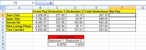
Figure 58
2. Type
an equal sign. See Figure 59:
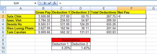
Figure 59
3. Notice
the equal sign in the formula bar as seen in Figure 60. (Don’t be alarmed that the name box has converted to an “Insert
Function” dropdown arrow with the SUM function showing– we’ll talk about this
later).

Figure 60:
The Formula Bar. The fx is a symbol from algebra that means “f of
x”, or function, or formula
4. Next,
using your “thick- white-cross” cursor, click in cell four to the left of F2
(cell B2). Like magic, Excel inserts the proper CELL REFERENCE after the equal
sign (see Figure 61). In addition, Excel shines the blue and yellow flashlight
around the cell B2 (these are the colorful marching ants that march around the
cell telling you that you have placed the CELL REFERENCE B2 behind the equal
sign).
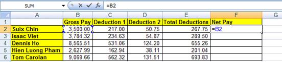
Figure 61
5. The
formula is now looking at a cell that is four cells to the left of F2 – looking
at the cell named B2 which holds Suix Chin’s Gross Pay. Because our goal is to
calculate Net Pay, we still have to subtract the Total Deductions.
6. Type
a minus sign, then using your “thick-white-cross” cursor, click in cell E2,
which is one cell to the left of F2. You should see this (Figure 62):
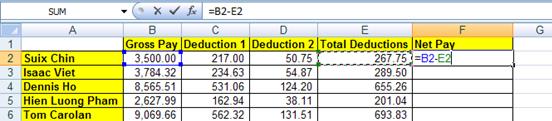
Figure 62
7. Hold
the Ctrl key, and then tap the Enter key once. This is what you should see (Figure 63):
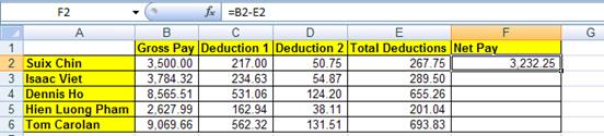
Figure 63
8. You
have just created your first calculating formula in Excel by using the equal
sign as the first character in a cell. Although the cell F2 displays the take
home pay of 3,232.25, what is actually in the cell can be seen in the formula
bar. Our formula reads: please look at Suix Chin’s Gross Pay (four cells to the
left in B2) then subtract the Total Deductions (one cell to the left in E2).
9. We
have creating our first calculation in Excel, and what we actually created is
called a formula. Because the equal sign is the first character in the cell we
told Excel to create a formula. If there was no equal sign, there would be no
formula. In addition, we used CELL REFERENCES. CELL REFERENCES are our way of
telling our formula to look into a different cell and use that value in our
formula!
10. What would
have happened if you did not place an equal sign in the cell as the first
character but you still typed the rest of the formula (Figure 64)? Excel would obey
you and not create a formula, but instead place the typed text “B2-E2” in the
cell.
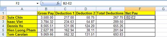
Figure 64
11. What would
happen if you type the number for gross pay and the number for total deductions
in the formula instead of the cell references? Here is an example of this
situation, however, please burn this image into you brain as something you
should NEVER do (Figure 65):
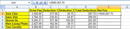
Figure 65
12. In Figure 65
Excel will obey you and calculate an answer. However, if you want to become
even moderately efficient with using Excel, NEVER TYPE NUMBERS THAT CAN VARY
INTO A FORMULA. When you enter numbers that can change (or text) into formulas
instead of references to other cells:
i.
Editing the formulas later on can become nearly
impossible
ii.
What-if or scenario analysis becomes cumbersome
iii.
The true magic of Excel is greatly dimmed, as if a
magnificent rainbow that fills the sky with refreshing color is suddenly all
one color of grey.
13. Numbers
such as the number 12 that represents months is OK to type into a formula.
Similar numbers would be things like 7 days in a week, 24 hours in a day.
The second magic character in Excel is the Ampersand (more
commonly known as the “and” character) “&”. This character joins the
content from two or more cells and places them all into one cell. To see an
example, click on the sheet tab named “Ampersand”.
Here are the steps to join
the words “Your” and “Name” and place them into one cell.
1. In
cell A1 type “Y o u r” (letters Y, o, u, r, space). You should see this (Figure
66):
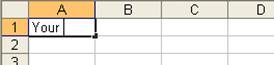
Figure 66
2. Hit
Tab. In cell B1 type “N a m e” (letters N , a, m, e), and then Tab. You should
see (Figure 67):
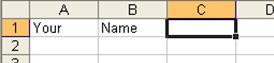
Figure 67
3. In
cell C1 type the an equal sign (Figure 68):
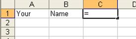
Figure 68
4. Hit
the left arrow key twice (Figure 69):
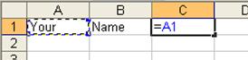
Figure 69
5.
Type the
Ampersand (Shift + 7) (Figure 70):
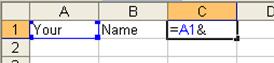
Figure 70
6. Hit
the left arrow key once (Figure 71):
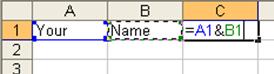
Figure 71
7. Hit
Ctrl + Enter (Figure 72):
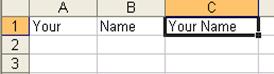
Figure 72
8. In
cell A1 type “Isaac ” and in cell B1
type “Newton” (Figure
73):
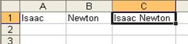
Figure 73
9. Now
try your own joining using the “&” (Figure 74):
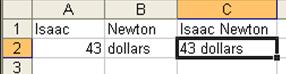
Figure 74
Note about the
Ampersand (&)“join” character: When you join two or more items using
the “&” in a formula, Excel treats the result as Text (in computer
programming language it is referred to as a “text string”). In other words,
Excel thinks that the formula result is a word, not a number. This becomes
important later when we need to distinguish between text and numbers.
Keyboard shortcut
Note:
Method of placing cell references in formula after you have placed an equal
sign as the first character in the cell: 1) use mouse to click on cell, 2) use
arrow keys to move to cell reference location, 3) type the cell reference
(higher probability of error)
Here are the steps to
calculate a monthly interest rate on a loan
1. Click
on the sheet tab named “Formulas”
2. As
seen in Figure 75, click in cell B2 and
type an equal sign. By typing the equal sign, you are telling Excel that you
are creating a formula in cell B2.
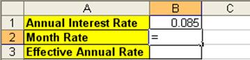
Figure 75
3. Click
the up arrow key (in between the letter keys and the number keys). By typing
the up arrow, you are telling Excel that you would like the formula to look
into the cell “one above” B2 and get the annual rate of .085. You should see
what is in Figure 76:
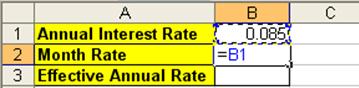
Figure 76
4. Notice
that by using the arrow key to select a cell reference, you save the time it
would take you to grab the mouse and click on cell B1.
5. Type
the division symbol “/” and the number 12 (12 months in a year does not vary so
that fact that this is a number does not violate Rule #6). See Figure 77:
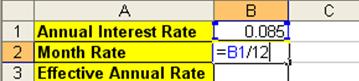
Figure 77
6. Tap
Enter. Taping the Enter key puts the formula in the cell and moves the cursor
one cell below B2 to the cell B3. The monthly rate displayed in the cell can be
seen in Figure 78:
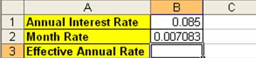
Figure 78
So far we have seen two keystrokes that tell Excel that the
formula is completed and we would like to have Excel show us the result. The
keystrokes “Ctrl + Enter” and “Enter” will officially enter the formula into
the cell. There are two other keystrokes that will officially enter the formula
into the cell: the “Tab” key will do it and Shift + Enter (Shift + Enter)
enters the formula and moves the cursor up – we will not use this one in this
book). These four keystrokes are the safest methods for putting the formula
into the cell. There are other keystrokes that work some of the time, but not
all the time. For safety and efficient formula creation we will only use Ctrl +
Enter, Enter, Tab or Shift + Enter to enter formulas into cells. If we use only
four keystrokes to place formulas in cells we can avoid unintended cell
reference insertion that can cause our formula to be inaccurate.
To enter a formula into a cell:
- Use “Ctrl + Enter” to
place the formula in the cell and select the cell with the formula
- Use Enter to place the
formula in the cell and select the cell directly below the cell with the
formula
- Use Shift + Enter to
place the formula in the cell and select the cell directly above the cell
with the formula
- Use Tab to place the
formula in the cell and select the cell one to the right
7. In
Cell B3, type: “=(1+”, as seen in Figure 79:
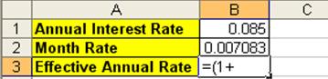
Figure 79
8. Click
the up arrow once, then type: “)^12-1”
as seen in Figure 80 ( ^ symbol = Shift +
6):
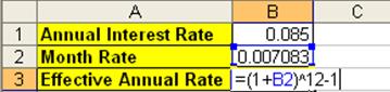
Figure 80
9. We
do not violate rule # 6 (DO NOT TYPE DATA THAT CAN VARY INTO A FORMULA) by
typing the 1, 12, and 1 into these formulas. For calculating the annual
effective rate from a month rate these numbers do not vary!
10. Click Tab.
You should see this (Figure 81):
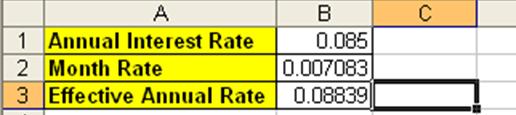
Figure 81
11. But what is
that “^” symbol mean? See the arrows in Figure 82
on the next page.


Figure 82
As seen in Figure 82, we will have to learn the Arithmetic
operation signs in Excel. In addition, we will have to learn the order of
operations in order to avoid analysis mistakes. For example, what is the answer
to 3 + 3 * 2? Is it 12 or is it 9? Because Excel knows the order of operations,
we must also know the order of operations so we can calculate correctly. For a
refresher in the order of operations, read Figure 82.
Here are the steps to practice
math and the order of operations:
1. Click
on the sheet tab named “Math (2)”. You should see this (Figure 83):
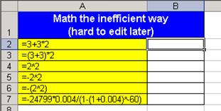
Figure 83
2. Click
in cell B2 and type the formula “=3+3*2”. You should see this (Figure 84):
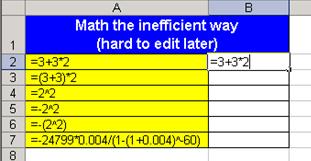
Figure 84
3. Looking
at the examples of formulas in column A, create the remaining formulas in
column B. When you are done you should have these results (Figure 85):
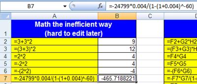
Figure 85
4. The
problem with what you just did (Figure 83,
Figure 84, Figure 85), is that editing the formulas later is inefficient when
compared to a method that employs cell references. Our next example will employ
cell references.
5.
Click in cell E2 and type an equal sign “=” (Figure 86).
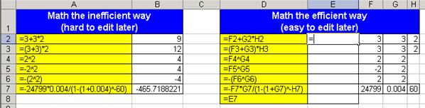
Figure 86
6.
Click the right arrow key, as seen in Figure 87:
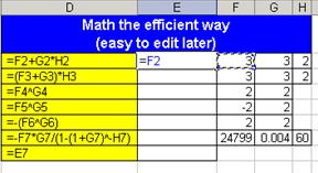
Figure 87
7.
Type “+”, as
seen in Figure 88:
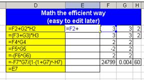
Figure 88
8.
Click the right arrow key twice, as seen in Figure 89:
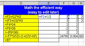
Figure 89
9.
Type the “*”, as seen in Figure 90:
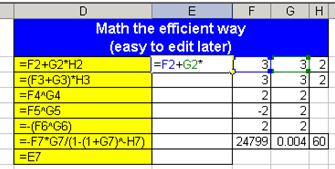
Figure 90
10. Click
the right arrow three times, (Figure 91):
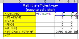
Figure 91
11. Hit
Enter. The answer should be 9.
12. In
Figure 92 the heading says “Math the
efficient way”. The efficiency comes from the fact that it is easy to edit
these formulas because you have utilized cell reference that point to numbers
typed into cells. Change the number in cell F3 to 12 and watch your formula
change (Figure 92):
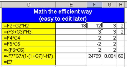
Figure 92
13. Look
at the formulas in column D) and create the corresponding formulas in column E.
When you are done you should see this (Figure 93):
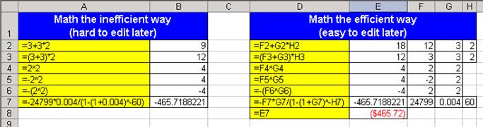
Figure 93
14. But
what is going on in cell E8? How come when cell E8 looks at cell E7 it shows us
a dollar figure? The answer comes from formatting. We will talk about
formatting later (this is exciting foreshadowing)…. For the time being we have
been taking about the equal sign, ampersand sign, numbers, cell references and
math operators: these are all components of formulas. We will now formally
define a formula in Excel è.
Definition of a
formula: Anything in a cell when the first character is an equal sign.
(The long version: anything in a cell or formula textbox
when the first character is an equal sign and the cell is not preformatted as
Text.)
Advantages of a
formula: You are telling Excel to do calculations, look into another cell,
create text strings, or deliver a range
How to create a formula: Type “=,” followed by:
1. Cell
references (also: names and sheet references)
2. Operation
signs
3. Functions
4. Text
that is in quotes (ex: “For The Month Ended”)
5. Ampersand
symbol: &
i.
To combine information from different cells, text in
quotes, or functions use the ampersand: &
1. Example:
="For The Month Ended "&B5
6. Numbers
i.
The only numbers that ever go in a formula are numbers
that will never change (such as the number of months in a year)
ii.
How to enter a formula into a cell: hit one of the following:
7. ENTER
8. Ctrl
+ Enter
9. Tab
10. Shift
+ Enter
Here are the steps to
create five formulas:
1.
You are currently looking at the sheet tab named “Math
(2)”. Make sure that you are in this sheet
2.
To use a keyboard shortcut to move two sheets up (back
toward the first sheet), hold down Ctrl, then tap the “Page Up” key twice (the
“Page Up” and “Page Down” keys are near the Home key).
Ctrl + Page Up è
moves you up through the sheets (toward the first sheet)
Ctrl + Page Down moves you
down through the sheets (away from the first sheet)
3.
You should now be located in the sheet tab named
“Formulas”
4.
Create the following formula (as seen in Figure 94). Efficient key strokes are: “=”, up arrow
twice, “-“, up arrow once.
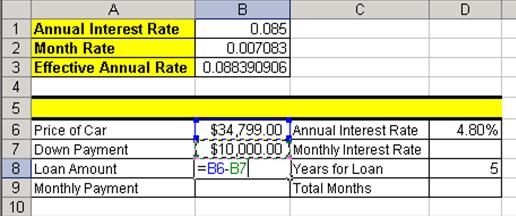
Figure 94
5.
Hit Tab twice, Arrow up and create this formula in D7 (Figure
95):
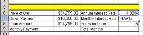
Figure 95
6.
The 12 represents months in a year and does not change
and so it is efficient to type this number into a formula
7.
Hit Enter twice and create this formula in D9 (Figure 96):
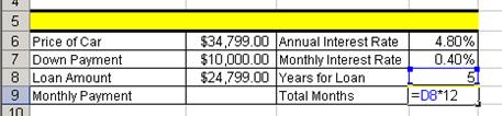
Figure 96
8.
Click in cell B9 and create the formula as seen in Figure
97. After you create it, hold Ctrl, then
tap Enter.
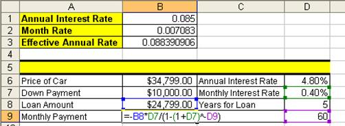
Figure 97
9.Click in cell A5. The cell is merged
and centered and so the formula will be created in the middle of the range. Create
the following formula as seen in Figure 98:
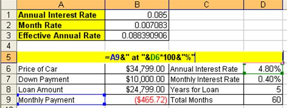
Figure 98
10. This
formula combines cell references, text in quotes and a calculation all joined together
with the Ampersand “&”. The resulting label for our calculations can be
seen in Figure 99:
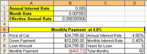
Figure 99
11. The
efficiency and beauty of building a spreadsheet in this manner is revealed when
we change the source data and then watch our formulas change automatically.
12. Click in cell B6 and change the price of the car to
50,000 (type 50000), then hit Tab twice. (Figure 100):
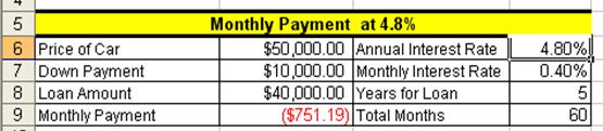
Figure 100
13. Notice
that the preformatted cells formatted the “50000” to appear as
“$50,000.00”. Also notice that our formulas for Loan Amount and Monthly Payment
updated.
14. Verify
that you are in cell D6 and then type “6” and then hit Enter (Figure 101):
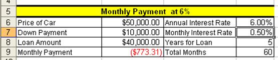
Figure 101
15. Notice
that the three formulas that were dependent on the Annual Interest Rate all
updated when we changed the rate. This ability to check different scenarios
without much effort is at the heart of using Excel efficiently. We always want
to strive to build our spreadsheets efficiently so that they are easily edit-customizable
at any time! By typing the numbers that can vary into cells and referring to
them using cell references in our formulas we have accomplished Excel
efficiency and fun!
16. Look in the lower left corner of Figure 102 and find the scroll arrow for sheet tabs.
The little black triangle turned on its side means show me one more sheet tab.
The little black triangle turned on its side with an extra vertical line means
take me all the way to the last and/or first sheet tab.

Scroll arrow that reveals more sheet tabs
|
|

Figure 102
17. Click
the sheet tab scroll arrow twice as seen in Figure 103:


Figure 103
18. You
should see a few more sheet tabs exposed. The sheet tab “Formulas” is still
selected, even though we see a few more sheets exposed (Figure 104):

Figure 104
19. Move
to the sheet tab named “Functions” by either clicking on the sheet tab named
“Functions”, or by Holding Ctrl, then tapping the “Page Down” key three times.
You should see this (Figure 105):
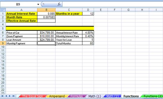
Figure 105
20. Click
in cell B9. What if we want to calculate the monthly payment for our car loan,
but we do not know that math formula? Luckily there are built in “Functions”
that know how to do this – as long as we can tell the Function what the monthly
rate, number of months and present value of our loan is, the function will do
the rest!
What are functions? Built in code that
will do complicated math (and other tasks) for you after you tell it which
cells to look in
Examples:
SUM function
(adds)
AVERAGE function
(arithmetic mean)
PMT function
(calculate loan payment)
COUNT
function (counts numeric values)
COUNTA
function (counts non-blank cells)
COUNTIF
function (counts based on a condition)
ROUND
function (round a number to a specified digit)
IF function (Puts one of two items
into cell depending on whether the condition evaluates to true or false)
Here the steps to practice
with many new Functions:
1. Click
in cell B9 and then click the fx button
(Insert function button) in the formula bar (Figure
106). (Keyboard
shortcut: Shift + F3 = Open Insert Function
dialog box)
Formula bar: from here to here
|
|

fx button è the
insert function button
|
|


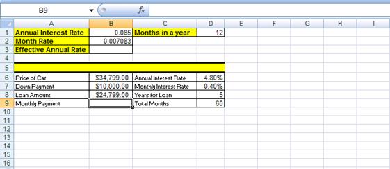
Figure 106
2.
The Insert Function dialog box looks like this (Figure 107):
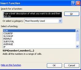
Figure 107
1.
There are five key parts to the Insert Function dialog
box:
1.
Search
2.
Category
3.
Select function
4.
Description of selected function
5.
Help
2.
Click in the search for a function text box and type
“monthly car payment” then hit Enter (Figure
108):
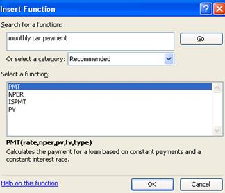
Figure 108
3.
In the select a function list the first function
selected is “PMT”
4.
Below the list is the description: “Calculates the
payment for a loan based on constant payments and a constant interest rate.” This
sounds perfect for our need. But let’s check the others to make sure that there
is not something even better. Click on “NPER.” Figure 109 shows the description
of this function:
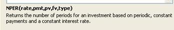
Figure 109
5. After
looking at each function, click back on the PMT function because, amongst the
four options, it fulfills our goal most satisfactorily. Descriptions are the
key to the Insert Function dialog box. You can find the most amazing functions
that will do all the calculating for you if you just spend a little time “hunting”
(looking through the list of functions).
6.
Because “hunting for the right function is the key to
learning about all the wonderful built-in functions, another way is to “hunt”
using the “All” category.
7.
Click the down-arrow next to “Select a category” and
point to All (Figure 110):
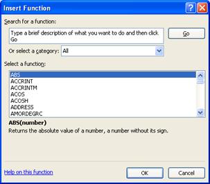
Figure 110
8.
Most of the functions have common sense names. See if
you can find a function that will calculate “Absolute value”, “Geometric mean”,
“Average”, “Straight-line depreciation”. All four of these can be found by
hunting for those words in the list.
9.
Absolute value (Figure 111):
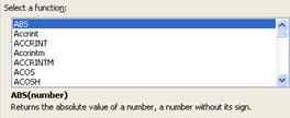
Figure 111
10. Geometric
mean (Figure 112):
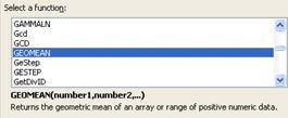
Figure 112
11. Average
(Figure 113):
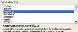
Figure 113
12. Straight-line
depreciation (Figure 114):
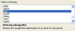
Figure 114
13. Now, find
the PMT function again. (Figure 115):
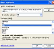
Figure 115
14. Double
click the highlighted PMT function to open the Functions Arguments dialog box (Figure
116):
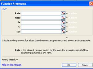
Figure 116
15. The
arguments “Rate” “Nper” and “Pv” are in bold and the most commonly used variables for this
function and are required for the function to give you a result. The “Fv” and
the “Type” are not in bold and are not required. There is a description for
each argument that will help you figure out how to use the function. In
addition, “Help on this function” (bottom lower left corner of Figure 116) is amazing! If you click that link it will
give you a full description and example of how to use this function. The help
looks similar to this (Figure 117):
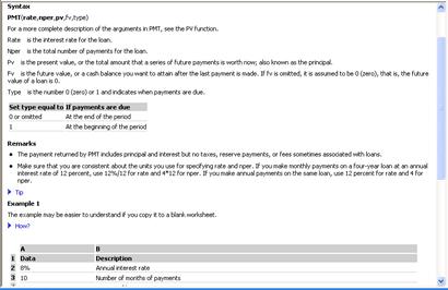
Figure 117
16. If you
opened up the help, close it. Make sure your curser is in the argument box for Rate, then click in cell D7 (Figure 118):

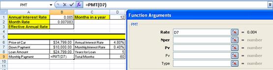
Figure 118
17. Notice that
when you click on cell D7 the value is shown to the right side of the argument
box.
18. Hit Tab to
move to the next argument box, click in cell D9, Hit Tab, Click in cell B8 (Figure
119):
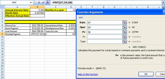
Figure 119
19. In Figure
119 notice:
1. Each
argument box has a cell reference (this makes it easy to edit later)
2. To
the right of each argument box that the variable amount is shown
3. The
formula result is shown in two different locations (can you see both?)
4. The
formula bar shows that Excel has placed an equal sign in the cell for you, that
the name of the function is in the formula and that the three cell references
(arguments) are separated with commas.
20. Click OK.
The result is the same as when we made our calculations before without the use
of an Excel function. (Figure 120):
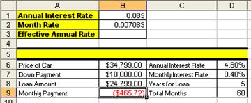
Figure 120
21. Click in
cell B3, hold the Shift key and tap the F3 key and then use the Insert Function
dialog box to find a formula for calculating the Effective Annual Rate. The
result should look like this (Figure 121):
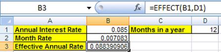
Figure 121
22. Click in
cell A5 and then hold the Shift key and tap the F3 key. In the Search for a
function text box type “join text” (Figure 122):
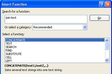
Figure 122
23. Create the
label for the Monthly Payment table (be sure to pay attention to the spaces
before and after the word “ at “) using the CONCATENATE function (Figure 123):
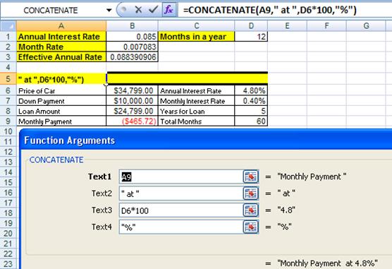
Figure 123
24. The result
looks like this (Figure 124):
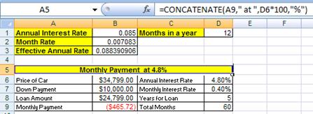
Figure 124
25. Type the
number “1”
into cell A13 and the number “2”
into cell A14. Then highlight the two cells (Figure 125):

Figure 125
26. Look at Figure
125. What is that little black box in the
lower right corner of the highlighted range? It is called the fill handle. It
is magic. Take your cursor and point to it until you see a cross hair (angry
rabbit). (Figure 126):

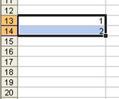
Figure 126
27. Click and
drag the angry rabbit down to A17. Just like magic Excel assumes you want to
add by 1 because the pattern of the number 1 and 2 is to always add 1. (Figure 127):
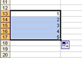
Figure 127
28. Click
in Cell A18. We are going to add all the numbers by using a SUM function. The keyboard shortcut for the SUM function is Alt + “=”.
29. Hold the Alt key, then tap “=” (Figure
128):
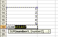
Figure 128
30. In Figure 128 we see that the SUM function tries to guess
what data we want to sum (it does not always guess correctly). It guessed
correctly this time and so we hit Ctrl + Enter (or if we are still holding the
Alt key we would tap “=” a second time. (Figure 129):
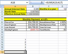
Figure 129
31. It is much more
efficient to use the SUM function, “=SUM(A13:A17)”, than it is to type in “=A13+A14+A15+A16+A17”.
In addition there is an added bonus to using a function that uses a range such
as A13:A17. Let’s take a look è
32. Point to
the row heading 15 and click to highlight the whole row (Figure 130):

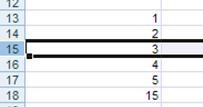
Figure 130
33. With the
row highlighted click on the Home Ribbon and point to Insert icon in the Cells
Group without clicking (Figure 131):

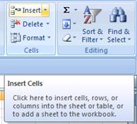
Figure 131
34. Notice that
a screen tip pops up to tell you what this icon button does.
35. Click the
Insert icon button and then click the Insert Sheet Rows button (Figure 132):
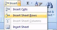
Figure 132
36. The result
is that you have inserted a row (Figure 133):
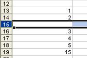
Figure 133
Note:
2007 Keyboard
shortcut Insert Row = Alt H + I + R
2003 Keyboard
shortcut Insert Row = Alt I + R
If
you want, use the 2003 version because it is shorter.
37. Click in
cell A15 and type the number “100”
and hit enter (Figure 134):
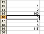
Figure 134
38. Notice that
the sum function updated
39. Click in
cell A19 and click the F2 key (Figure 135).
Keyboard shortcut for “Range Finder” = F2
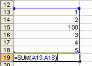
Figure 135
40. Range
Finder allows us to audit a formula after it is created. Look at the range we
have in Figure 135 (A13:A18). Now look at
the range in Figure 129. Our conclusion:
by using a function with a range our formula will update when we insert rows or
columns. If we had used the formula “= A13 + A14 + A15 + A16 + A17”, it would
not have updated when we inserted a row.
41. For more
practice with Functions go to the sheet tab named “Functions (2)”
42. Hover your
“thick, white-cross” cursor over cell A2, then click in cell A2, hold the
click, and drag your cursor to cell J9. This is how you highlight a range. The
range you have highlighted is A2:J9. (Figure 136):
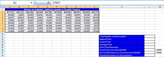
Figure 136
43. Click in
the Name Box (Figure 137):
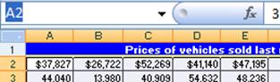
Figure 137
44. After you
click in the name box it will highlight the cell A2.
45. Type over
“A2” and replace it with “sd” (“sd” will stand for sales data). (Figure 138):
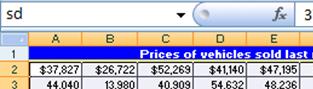
Figure 138
46. Then hit
Enter to register the newly named cell range. The cell range A2:J9 now has the
name “sd” When we create functions that look at that range we can now simply
type in “sd” instead of highlighting the range A2:J9
47. Click in
cell L11 and see if you can find a function that can count the number of cars
that were sold last month at Seattle Toyota. When you find it, your formula
result should look like this (Figure 139):
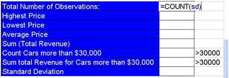
Figure 139
48. See if you
can find the remaining functions using your new “function hunting skills”
49. When you
are done you should see the same results that you see in column L in Figure 140 by using the formulas that you see in
column N in Figure 140.
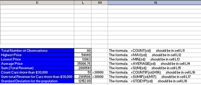
Figure 140
50. We have
been using cell references so often, that it is now time to investigate the
different types of cell references è
When we copy formulas that contain cell references to other cells, then we
need to understand that there are four types of cell references:
1. Relative
2. Absolute
3. “Mixed
Cell Reference with Column Locked” also known as “Column Absolute, Row Relative”
4. “Mixed
Cell Reference with Row Locked” also known as “Row Absolute, Column Relative”
It will only be possible to
understand these if we look at a few examples. Nevertheless, here are the
crucial facts about cell references:
1.
Relative Cell References Example: A1
No
dollar signs
Moves
relatively throughout copy action
“Relatively” means that if the formula
is looking at a cell reference that is three cells to the left, when you copy
the formula to any other cell, the cell reference will still be looking three
cells to the left.
2.
Absolute Cell References Example: $A$1
Dollar
signs before both:
Column
designation = A
Row
designation = 1
“Absolute”
means that if the formula is looking at a particular cell reference, when you
copy the formula to any other cell, the cell reference will still be looking at
that particular cell reference.
If the Absolute
Cell reference is $A$1, the formula will always look at cell A1. It is as if
the formula is locked on the cell A1 throughout copy action
“Locks cell reference when copying it
horizontally and vertically”
3.
“Mixed Cell Reference with Column Locked” Example: $A1
Dollar
sign before column designation
Remains
absolute or locked when copying across columns
Remains
relative when copying across rows
“Locks cell reference when copying it
horizontally, but not vertically”
4.
“Mixed Cell Reference with Row Locked” Example: A$1
Dollar
sign before row designation
Remains
absolute or locked when copying across rows
Remains
relative when copying across columns
“Locks cell reference
when copying it vertically, but not horizontally”
Keyboard shortcut F4 key: Toggles
between the four types of cell references
When creating formulas
with cell references, ask two questions of every cell reference in formula:
Q1:
What do you want it to do when you copy it horizontally?
Is
it a relative reference? OR
Is
it an absolute or locked reference?
Q2:
What do you want it to do when you copy it vertically?
Is
it a relative reference? OR
Is
it an absolute or locked reference?
Here are the steps to
learn about the four cell references:
1. Go
to the sheet tab named “Cell References” and click in cell C3 and create the
formula shown in Figure 141. The formula
calculates a proportion or percentage of the whole (depending on how it is
formatted). In our example we are comparing Tina’s score (82 parts of the 100
whole) and comparing it to the total possible points (100 points – the whole).
If you look ahead to creating the formulas for Sue and Chin and Hien, all their
“parts” will have to be compared to the “whole”.
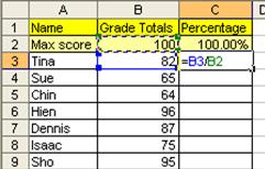
Figure 141
2. Hold
Ctrl, then tap Enter. You should see that the proportion of points that Tina
earned is .82 (Figure 142):
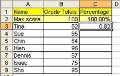
Figure 142
3.
To format the number “.82” as a percentage,
highlight cell C3, click the Home Ribbon and then click the % icon button in
the Number Group. (Figure 143). Remember
82% is not a number. Underneath in Excel’s code (just like any other
calculator), Excel sees the number “.82” even though it is formatted with a %
symbol and even though what we see in the spreadsheet is 82%:
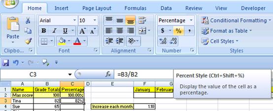
Figure 143: Notice the Screen Tip that let’s us
know the keyboard shortcut for this format.
4. Highlight
the range C4:C9 and then use the keyboard shortcut to add the % style (Ctrl +
Shift + %): this pre-formats the cells with the percentage format (Figure 144):
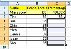
Figure 144
5. Click
in C4 and create the formula for calculating Sues’ percentage grade (Figure 145):
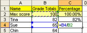
Figure 145
6. Continue
until you have created the percentage grades (Figure 146):
Figure 146
7. What
we just completed did not require that we know anything about the four
different cell references. However, what we did was inefficient. There is a way
to create all those formulas by just creating one formula in cell C2 and then copying
it down through our range. We will have to learn how to “LOCK” or make
“ABSOLUTE” some of our cell references. If we can learn how to do this, it will
make tasks such as this easier to complete and will result in few errors. In
addition, many of the most advanced Excel Features and tricks are only possible
if we learn about these four cell references.
8. Highlight
the range C2:C9 and then hit the delete key (Keyboard
short cut: Delete key = delete cell content but not format) (Figure 147):
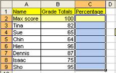
Figure 147
9. Click
in cell C2 and create the following formula (Figure 148):
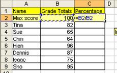
Figure 148
10. Figure 148 shows a fraction B2/B2. For clarification
of terms: Numerator means the top of the fraction and Denominator means the
bottom of the fraction.
11. Now think
about this: the numerator B2 needs to always look one cell to my left and the
denominator B2 always needs to be locked on B2. We have to let Excel know that
the two B2s are different.
The
numerator B2 needs to always look one cell to my left
i.
This is called a relative cell reference
ii.
Relative to the cell the formula sits in, the cell
reference always needs to look one cell to the left
iii.
For our example the “one-to-the-left” B2 will be
entered into the formula as B2
The denominator
B2 always needs to be locked on B2
i.
This is called a locked or absolute cell reference
ii.
The secret code we need to put into our cell reference
to let Excel know that the cell is locked in the “$” sign. Why the dollar sign?
No reason – just think of it as the secret code).
iii.
But where do we put the secret code? The answer depends
on which direction you will be copying the formula. In our case we will be
copying up-and-down (vertical direction), across the rows (and rows are
numbers), so the secret code goes in front of the Number 5.
iv.
For our example the “LOCKED” B2 will be entered into
the formula as B$2
12. Very
carefully, place your cursor in the middle of the denominator B2 and click the
F4 key twice. The first tap of the F4 key will put two dollar signs into the
cell reference, then the second tap of the F4 key will toggle to the next cell
reference which has only one dollar sign in front of the number 2. See Figure 149:
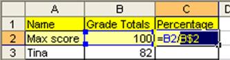
Figure 149
13. Hold Ctrl,
then tap Enter. You should see this (Figure 150):
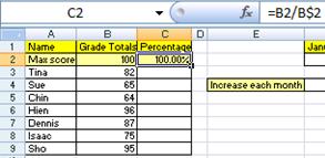
Figure 150
14. Point to
the fill handle and with your angry rabbit, double-click the fill handle to copy
the formula down to cell C9 (Figure 151):
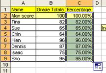
Figure 151
15. In Figure 151, notice that it copied the yellow cell fill
color formatting down with the formula. Take you cursor and click on the blue
smart tag, then click on Fill Without Formatting (this great feature copies
only the formula) (Figure 152):
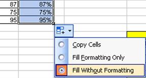
Figure 152
16. Click in cell
C9 and audit the formula (F2 key) to make sure that you actuality did create 8
formulas, but only had to create one formula which you then copied down (Figure
153):
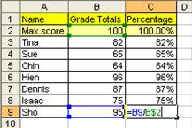
Figure 153
17. Click in
cell G2 and create the formula seen in Figure 154.
Because the January 1000 amount will be increased by 10% each month, we need to
multiply (1 + .10) or 1.10 by each previous month’s amount. But notice that the
cell reference F2 is actually always going to be looking at the cell “one-to-the-left”
(relative cell reference = F2) and the cell reference F4 will always be
“locked” on F4 when copying it side-to-side, across the columns (columns are
letters), so the secret code goes in front of the letter (locked copying it
across the columns = $F4)

Figure 154
18. Very
carefully, place your cursor in the middle of the F4 and click the F4 key three
times (Figure 155):
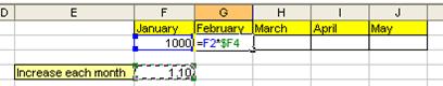
Figure 155
19. Hit Ctrl +
Enter. Point to the fill handle and copy to formula to J2 (Figure 156):
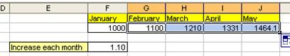
Figure 156
20. Click in
cell J2 to audit the formula with the F2 key (Figure 157):
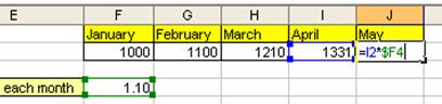
Figure 157
21. Look in Figure
158 at the table titled “What will your
Pension be worth when you retire?” We would like to estimate what our pension
will be depending on the annual rate that we earn and how many years we save
for retirement. The trick here is that we don’t want to type 54 formulas. We
would like to create the whole “sea of formulas”, G13 to L21, by creating only
one formula in cell G13 and then copying it to the remaining cells.
22. Click in
cell G13 and type “=FV(“. The screen tip will come up to help you with the arguments
for this function. To calculate our retirement funds we will need to assume an
annual rate “rate”, the number of
years that we deposit money “nper”
and a yearly deposit amount “pmt” (Figure
158):
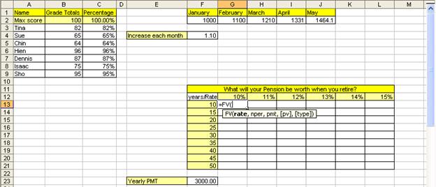
Figure 158
23. Click on
cell G12 (Figure 159):
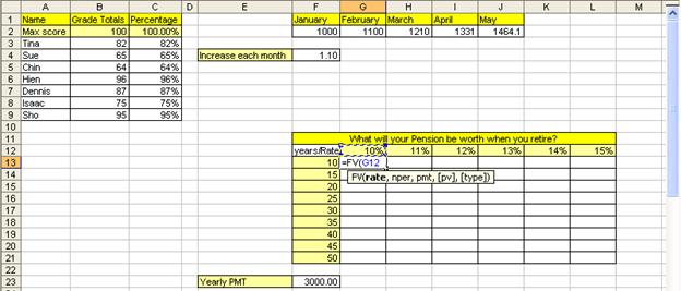
Figure 159
24. Can you see
in Figure 159 that we will need to use
the 10% for all the formulas in column G? Can you also see that when we copy
the formula over to column H we need to use the 11%? This means that we need
the cell reference locked (absolute) when we are copying the formula down, or
vertically, or across the rows: the row reference needs to be locked! However,
when we copy the formula to column H the cell reference should not be
locked (absolute) when we are copying the formula to the side, or horizontally,
or across the columns. The column reference is not locked: it is relative.
25. Because we
want to lock (absolute) this cell reference when we copy the formula down, across
the rows, we need the “$” sign in front of the number. Because we want this
cell reference to move relatively as we copy the formula to the side, across
the columns, we do not need the “$” sign in front of the letter. Cell reference
= G$12 è
hit F4 twice (Figure 160):
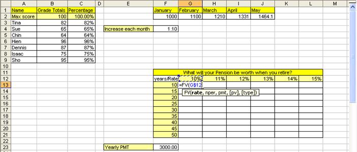
Figure 160
26. Type a
comma, click on F13, and hit F4 three times.
27. We hit F4
three times because we want this cell reference to move relatively as we copy
the formula down, across the rows, and we want the cell reference locked
(absolute) as we copy the formula to the side, across the columns. Cell
reference = $F13 è
(Figure 161):
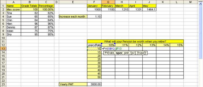
Figure 161
28. Type a
comma, type a minus sign, click on cell F23, and hit F4 once, type a close
parenthesis.
29. Because we
want to use the cell reference F23 in every cell when we copy this formula, we
want the cell reference locked in all directions. The dollar sign in front of
the column reference “F” locks the cell reference when copying the formula to
the side, across the columns. The dollar sign in front of the row reference “23” locks the cell reference
when copying the formula down, across the rows. Cell reference = $F$23 è
(Figure 162):
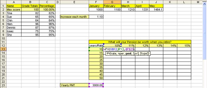
Figure 162
30. Hold Ctrl, and
then tap Enter. Point to the fill handle and double-click the fill handle to
copy the formula down to cell G21 (Figure 163):
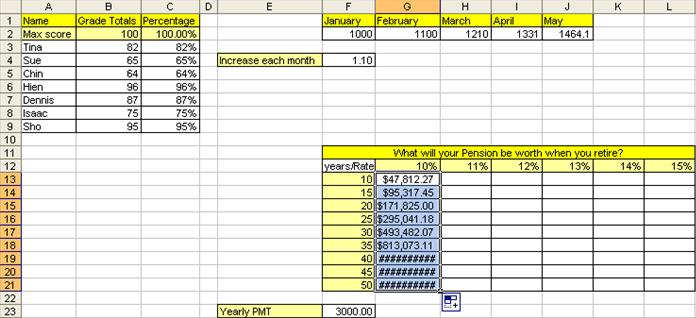
Figure 163
31. Don’t be
alarmed by the pound signs. They are just saying: “Please expand the column so
this big number has room to show itself.” Point between the two column headings
G and H and double click to expand the columns. You should see this (Figure 164):
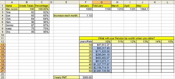
Figure 164
32. Now point
to the fill handle in the lower right corner for the entire range, then click
and drag to L21. Notice that many pound signs appear. Highlight the column
headings from H to L by clicking on the columns heading H and dragging to L.
Then double-click between the column headings H and I to expand the columns (Figure
165):
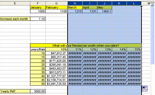
Figure 165
33. Our result
is that 54 formulas were created by enter just one formula, adding the correct
cell references and then copying the formula in two-steps (first down, then
over) (Figure 166):
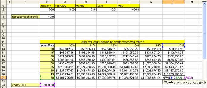
Figure 166
34. For more
practice with cell references, click on the sheet tab named “Multiplication
Table and see if you can create 144 formulas by enter just one formula, adding
the correct cell references and then copying the formula in two-steps.
In the last few examples we saw what
happens to cell references when we copy a formula that has cell references. Now
we need to see what happens when we move a formula that contains cell
references. Copy means copy the formula from a cell or range of cells, leave
the formula in the original location, and then paste the formula in some other location.
Move means cut the formula from a cell or range of cells, it will no longer be
located in the original location, and then paste the formula in some other location.
Here are the steps to
learn about the difference between copying and moving a formula with cell
references.
1. Click
on the sheet tab named “Copy and Move.” Click in cell B6 and follow the
instructions listed in cell B5 (Figure 167):
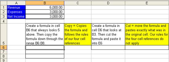
Figure 167
2. Figure
168, Figure 169 and Figure 170 illustrate
that when you copy a cell reference that has a relative cell reference component,
the cell reference changes relatively. In Figure 168 we see a formula that is looking into cell B1. In Figure 170 we see a formula that is looking into cell
B3. When we copied the formula, the cell reference moved relatively – it
actually did exactly what we told it to do, namely, “always look five above”.
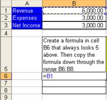
Figure 168
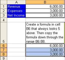
Figure 169
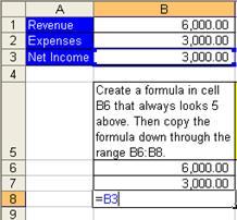
Figure 170
3. Now
let’s look at what happens when we cut a formula with a relative cell reference
and paste it somewhere else.
4. Click
in cell D6 and create the formula “=B3” (Figure 171):
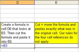
Figure 171
5. Hold
Ctrl, then tap Enter (Figure 172):
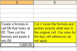
Figure 172
6. Ctrl
+ X (keyboard shortcut for Cut), hit Tab (Figure 173):
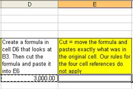
Figure 173
7. Ctrl
+ V (Figure 174):
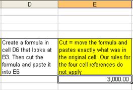
Figure 174
8. Hit
F2 (Figure 175Figure 174):
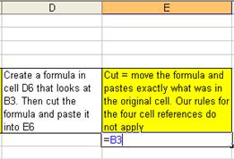
Figure 175
9. Compare
Figure 171 and Figure 175. When you cut a formula with a relative
cell reference component and paste it into a new cell, the formula does not
change – it actually moves the cell references exactly as they were in the
original cell and pastes them in the new location. This is because when you
move, you do not change anything; you simply put the formula, intact, in a new
location.
10. Wow!
Knowing the difference between moving and copying formulas is very helpful in
our pursuit of efficient spreadsheet construction. Let’s practice copying a
formula with relative cell references another time before we move on to the
next topic è
11. Navigate
back to the sheet tab named “The Equal Sign” by holding the Ctrl key, and then
tapping the Page Up key nine times. You should see this (Figure 176):
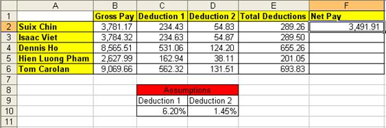
Figure 176
12. Click in cell F2. Hit the F2 key (Figure 177). Look at
the formula in cell F2. Can you say what type of cell references they are? Can
you say what will happen to the formula when you copy it down from F2 to F6?
The formula in cell F2, “=B2-E2”, uses relative cell references and so when you
copy it down the cell references will move relatively. The formula actually
reads: “always look four to the left and subtract one to the left”.
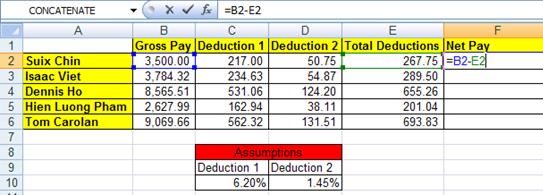
Figure 177
13. Hold Ctrl,
then tap the Enter key. Point to the fill handle and with your cross hair
(angry rabbit) and then double click the fill handle. The double click on the
fill handle tells the formula to copy down as long as there is cell content in
the cell directly to the left (Figure 178):
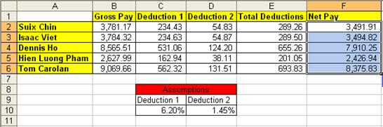
Figure 178
14. Click in
cell F6 and hit the F2 key (Figure 179).
Because the cell references are relative and because we copied the formula, the
formula, “=B6-E6”, looks different, but really it is the same formula, namely:
“always look four to the left and subtract one to the left”.
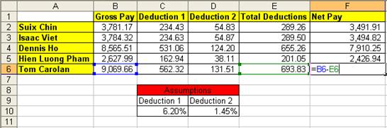
Figure 179
15. Look at Figure
179. What is the word “Assumptions”
across C8 and D8 mean?
16. Click the
Esc key to remove the range finder in cell F6. Click in cell C2 and then hit
the F2 key (Figure 180). We can see in
our formula that Deduction 1 is calculated by taking Suix Chin’s Gross Pay and
multiplying it by the tax rate of 6.20%. Because the tax rate of 6.20% can
change we have placed it in a cell and had our formula refer to it using a cell
reference. We have assumed that our tax rate is 6.20% and thus have placed it
into an assumption table. In our next section we will discuss the amazing power
of assumption tables: when you should use them, what to put in them, and how to
properly orientate them!
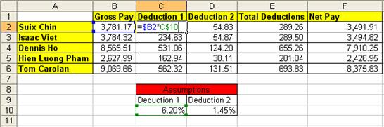
Figure 180
Our golden rule for assumption tables is: All data that can
vary (variable data) goes into a properly orientated assumption table. An
example of data that can vary is a tax rate. An example of that data that will
not vary is 12 months in a year. Remember: we don’t want to type data that can
very into a formula for three reasons:
- It is easier to edit or
change our formula later if the variable data it is not typed into the
formula (example: tax rate changes)
- It is more polite for the
spreadsheet user if the variable data can be seen on the face of the
spreadsheet. (For example, even if we were to create a formula with
variable data typed into the formula (such as “=$B2*.062”), when we came
back tomorrow to use the worksheet, we as the creator might not even
remember which formulas have variable data and/or what the variable data
is)
- What-if
or scenario analysis is significantly easier when an assumption table is
used. What-if/scenario analysis is simply when you change the variables to
see different formula results.
In addition to the ease with
which we can edit or locate variable data, assumption tables that are properly
orientated can reduce the number of formula that we will be required to type
into our spreadsheet. Proper orientation means the labels in the main table are
orientated (horizontally or vertically) in the same way as the labels in the assumption
table (horizontally or vertically), and that there is at least one blank row or
column between the main table and the assumption table. Also, you can format
the assumption table differently to distinguish it from the main table.
In this section about assumption tables we will learn:
1. When
to use them
2. What
to put in them
3. How
it is easier to locate and edit variable data
4. How
to properly orientate them!
5. How
to conduct What-if/scenario analysis easily
6.
How to bask in the amazing power of assumption tables!!
It will help if we work through
an example è
Here are the steps to
learn about assumption tables:
1. Navigate
to the sheet tab named “Assumptions” (Figure 181).
This table will be used to calculate the Net take home pay for a number of
employees. Notice that the calculated amounts for Commission on Sales, and
Gross Pay have already been calculated. Our goal is to calculate the three
payroll deductions (FICA, Medicare, and simplified Federal) and the Net Pay.
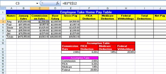
Figure 181
2. Click
in cell C3 and hit the F2 key. We can see the formula “=B3*E$12” ( Figure 182). Our first question we want to answer is:
when do we use an assumption table? We use an assumption table when our formula
contains variable data such as a commission rate or tax rate. In cell E3 we are
calculating the commission on sales that we pay each employee. Can this
commission rate change? You bet!
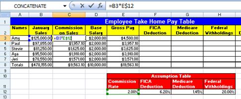
Figure 182
3. Hit
the Esc key. Click in cell E12. Our second question is: what do we put into an
assumption table? We put the variable data that we need for our formulas into
an assumption table. In Figure 183 we can
see that the commission rate of 1.25%, which we used in our formula, has been
placed into an assumption table. This enables easy editing and formula updating
later.
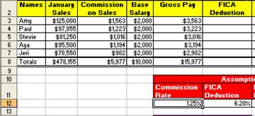
Figure 183
4. Now,
imagine that the boss just gave everyone a raise from 1.25% commission to 2%!
This leads to our third question: How easy is it to locate and edit variable
data? Very easy!
5. Type
2, then hit Enter (because the cell was preformatted with the percent style, we
did not have to type the % symbol). You should see the entire column of “Commission
on Sales changes (Figure 184). THAT WAS
EASY!! It is easier to change the variable data when it is on the face of the
spreadsheet that it is to look for it, hidden underneath, inside a formula! I
can already feel that vacation time adding up with all the time I will be
saving!
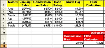
Figure 184
6. Click
in cell E12 and change the rate back to 1.25%. Our goal is still to calculate
the deductions and calculate take home pay
7. Click
in cell F3 and create the formula for calculating the FICA deduction. But wait!
Which assumption table should we use?
8. Is
the formula “=E3*F$16” (Figure 185) the
one to use?
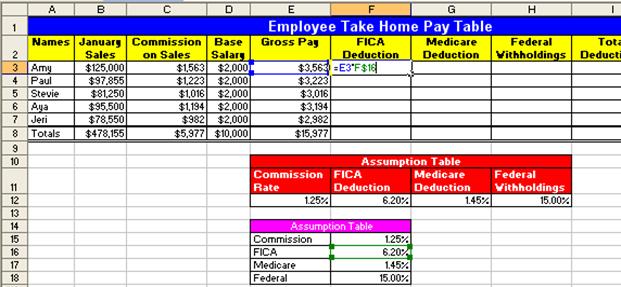
Figure 185
9. Or
is the formula “=$E3*F$12” the one to use?

Figure 186
10. The answer
to which formula to use (which formula is more efficient) leads to the fourth question:
what is the proper orientation for our assumption table? If we were to use the
formula as seen in Figure 185, “=E3*F$16”
we would have to create three separate formulas to make all our deduction
calculations. If we were to use the formula as seen in Figure 186, “=$E3*F$12” we would have to create only
one formula to make all our deduction calculations. This sort of efficiency is
exactly what we are striving for. But why does the formula using the variable
data from the assumption table that is orientated horizontally allow us to
create only one formula that will work for all our deductions? To see this,
let’s try both formula and see which works best.
11. You should
still have cell F3 highlighted. Create this formula: “=E3*F$16” (Figure 187):

Figure 187
12. Hold Ctrl,
then tap Enter. Point to the fill handle, and with the Angry Rabbit cursor,
copy the formula down through the range
F3:F7. Then click in cell F7 and hit the F2 key (Figure 188). You can see that the formula worked when we copied it down.

Figure 188
13. Hit Esc. Click
back into cell F3. Copy the formula to cell G3. Click in cell G3 and hit the F2
key to show the Range Finder. In Figure 189
we can see that the range finder shows that the cell reference for our tax rate
moved and is now looking into the cell G16. Because the orientation of the
assumption table is vertical (the labels for FICA, Medicare and Federal are
located one on top of the other) and the orientation of our main table is horizontal,
we would have to create three individual formulas in the cells F3, G3 and H3.
Notice that in Figure 189 that the range
finder moved to the right when we copied our formula to the right. This
indicates that if we had used the horizontally orientated assumption table that
formula would have calculated correctly è
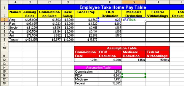
Figure 189
14. Click Esc.
Then Hold Ctrl, and tap the Z key three times (undo). Then create the formula “=$E3*F$12”
in cell F3 (Figure 190):
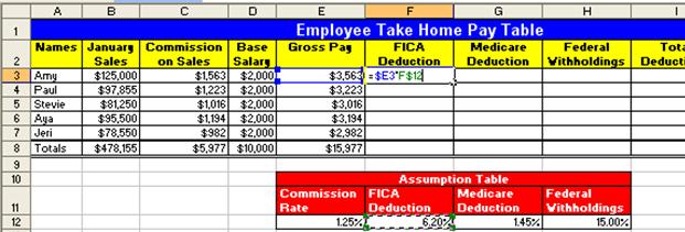
Figure 190
15. Hold Ctrl,
tap Enter. Ctrl + C (to copy formula). Hold Shift, then tap the Down Arrow key
4 times and the Right arrow key 2 times (highlights the range). Ctrl + V
(pastes formula). Click in cell H7 and hit the F2 key. In Figure 191 we can see that because we orientated our
assumption table correctly, it worked like MAGIC! We created the sea of
formulas in the range F3:H7, 15 formulas, but we only had to type in one
formula! This sort of efficiency is our goal!
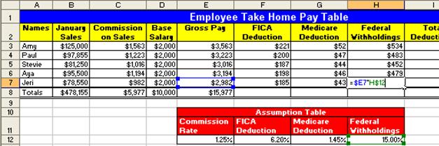
Figure 191
16. Hit Esc.
Highlight the range F3:I8 (Figure 192):
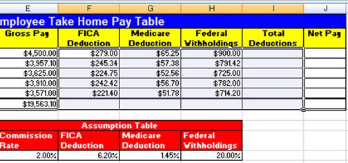
Figure 192
17. Hold Alt,
and then tap the Equal sign key “=” (Alt + = is keyboard shortcut for AutoSum).
As you can see in Figure 193, by
highlighting a range of values and one blank row below and to the right, the
Auto Sum feature knew what to add up. It doesn’t always add up the correct
amount, so let’s check to be sure. After selecting cells with the AutoSum and
verifying, the last cell we will check is cell I8 (Figure 193):
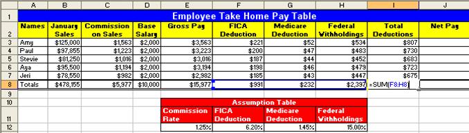
Figure 193
18. Highlight
the range J3:J8 (Figure 194). Notice that
when you highlight a range that one of the cells is white and the rest are a
light steel-blue color. The white cell is waiting for you to put a formula into
it. If you put a formula into cell J3 and then hold Ctrl and tap Enter, you
formula will go into all the cells highlighted è
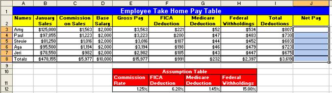
Figure 194
19. Create the
formula that will always take the value “five to the left and then subtract one
to the left in cell J3. Type ‘=”, tap the left arrow key five times, Type “-“,
tap the Arrow key once. You should see this (Figure 195):
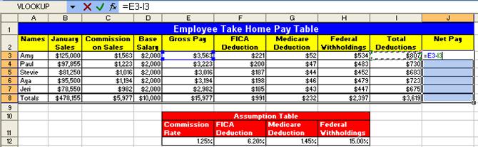
Figure 195
20. Hold Ctrl, and
then tap Enter. We see here that if you have a range
highlighted and you place a formula into the white cell, when you hold Ctrl and
tap Enter, the formula is placed into all the cells that are highlighted!
You should see this (Figure 196):
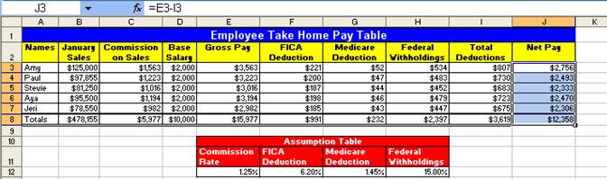
Figure 196
21. Our fifth
question is: How easy is what-if/scenario analysis when we use assumption
tables?
22. Click in
cell E12 and change the Commission rate to 2%. Click in cell H12 and change the
simplified Federal Withholding rate to 20%. Can you see how easy it is to say:
“What if I changed this; what would happen to our calculations and our
results?” (Figure 197):
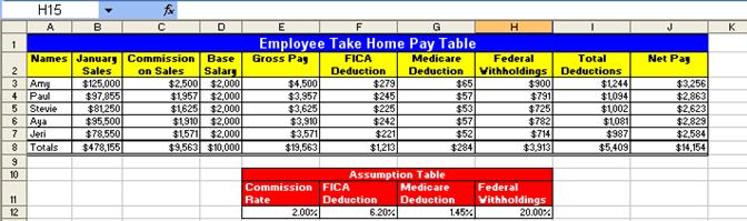
Figure 197
23. Our final
question about assumption tables is how can we bask in the amazing power of
assumption tables?
24. Imagine
your boss comes in and says: “we just added a new 2% deduction can you update
our calculating table?” You look over your shoulder and say: “Oh you mean like
this?!!” And with blistering speed you complete these steps è
25.  Click in any cell in column H, Tap
Alt, then tap I and then tap C (Alt + I + C is the keyboard shortcut for Insert
Column) (Figure 198):
Click in any cell in column H, Tap
Alt, then tap I and then tap C (Alt + I + C is the keyboard shortcut for Insert
Column) (Figure 198):

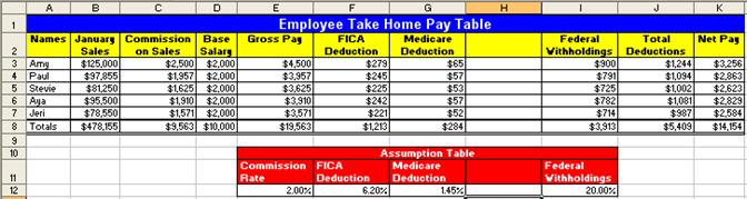
Figure 198: Alt + I + C is the keyboard
shortcut for inserting a column
26. Click in
cell H11 and type Pension. Hit Enter, then type 2% (Figure 199):
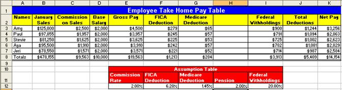
Figure 199
27. Highlight
the range G2:G8 and point to the fill handle in the lower right-corner. When
you see your Angry Rabbit, click and drag one column to the right. You are
done! 10 clicks and you have completely updated the table and you have amazed
your boss (who then promptly gives you a promotion)! (Figure 200):
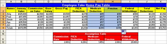
Figure 200
28. In Figure 200 we can see that the deduction formulas
updated because we used a properly orientated assumption table and mixed cell
references; we can see that the SUM function for totals in row 8 updated
because they were always looking to add the five above; and we can see that the
totals for Total Deduction updated when we inserted a column because it
utilized a range in its arguments! Wow, now we can have extra vacation time and
bask in the amazing promotion we received – all because of efficient use of
assumption tables, mixed cell references and range functions!
29. Highlight
the range K3:K8. To Increase the decimals, click on the Increase Decimal icon
in the Number Group on the Home Ribbon, or use the key board shortcut Alt + H +
0 twice. (Figure 201). Notice that the
total Net Pay is $13,762.64.
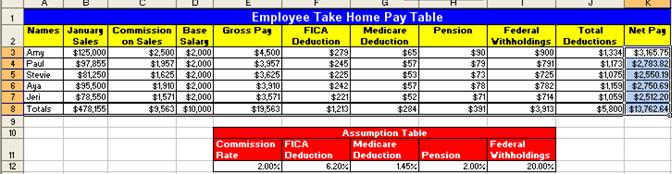
Figure 201
30. Click in
cell K8 and then hit the F2 key (Figure 202).
There is no way that $19,563 - $5,800 = $13,762.64. What is going on here? This
is one of the most common mistakes that people make in Excel. It is our job as
Soon-To-Be Excel Efficiency Experts (EEE), to know that this is caused by
formatting. What we often see in Excel is not actually what sits in the cell. We
must investigate further….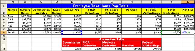
Figure 202
31. To prove to
ourselves that what is in the cell is different than what we are seeing on the
surface of the spreadsheet, highlight the range B3:K8 and increase the decimals
so that we see the decimals to the penny (Figure 203). We can see that what was really in the cell was numbers with
more decimal places than we were allowed to see!
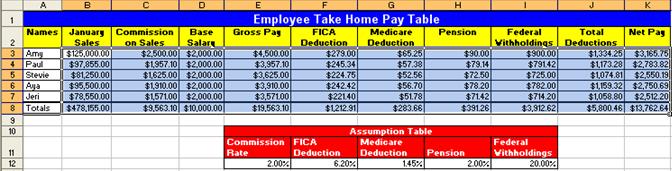
Figure 203
32. As you learn to work with Excel you must be vigilant
in the endeavor to always match the proper formatting with what actually sits
in the cell. This leads us to our next section about formatting.
We format cells with color, number
formats (such as currency), borders and other format so that we can better
articulate the message of our spreadsheet or printout of the spreadsheet. For
example in Figure 204 we can see that
formatting can help to communicate important information:
1. The
percentage format helps to communicate the number of parts for every 100 parts
2. The
accounting (similar to currency) format indicates that the Revenues, Expenses
and Net Income are in USA
dollars
3. The
double line under the Net Income communicates that this is the “bottom line”.
4. The
color helps to communicate that there are labels indicating what the numbers
mean
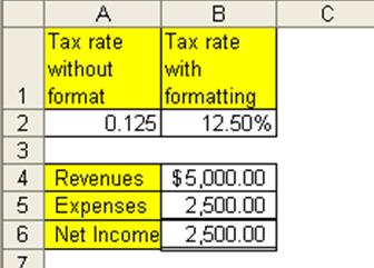
Figure 204
Here are the steps to
learn how to apply cell formatting
1. Navigate
to the sheet named “Formatting (2)”. Click in cell E2. Hold Ctrl, then tap the “*” key on the number pad (this
selects the table) (Figure
205):
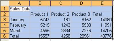
Figure 205
2. Click
the drop-down arrow to the right of the Border icon button in the Font Group on
the Home Ribbon. Then select the “All Borders icon from the drop-down list (Figure
206):
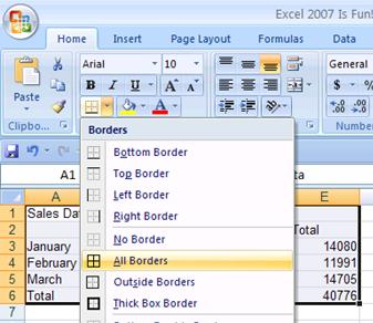
Figure 206
3. Highlight
the range A1:E1. Hold Ctrl key and tap “1” key (use the “1” below the F1 key not the “1” on the number pad). Ctrl + 1 opens the Format Cells dialog box (you could
also right-click the highlighted range and point to Format Cells) Once you have
the Format cells dialog box open click on the Alignment tab. See (Figure 207):
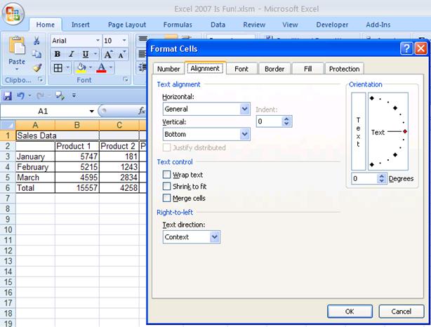
Figure 207
4. With
the Alignment tab selected, click the down arrow under Horizontal and
select “Center Across Selection” (Figure 208):
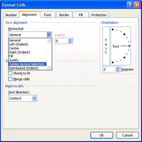
Figure 208
5. We
chose “Center Across Selection” instead of the more widely used “Merge and
Center”. “Center Across Selection” allows move universal structural changes
such as inserting columns/rows and moving, whereas the “Merge and Center”
sometimes will disallow such actions.
6. Click
the Font tab. Select “Poor Richard” font (or some other font), Bold style, Size
= 14, Color (of font) = White (Figure 209):
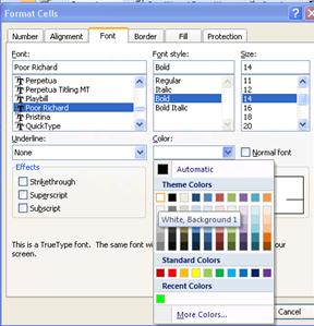
Figure 209
7. Click
on the Patterns tab and select a dark blue (Figure 210):
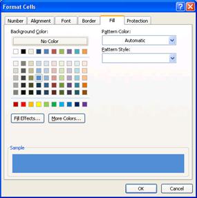
Figure 210
8. Click
OK (Figure 211):
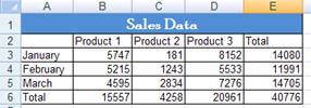
Figure 211
9. Highlight
the rangeB2:E2, Hold Ctrl, Highlight A3:A6 (By holding the Ctrl key you can
select cells that are non-adjacent. Click the Fill color button in the Font
Group on the Home Ribbon (Figure 212):
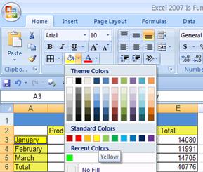
Figure 212
10. Highlight
the range B3:E6 (Figure 213)
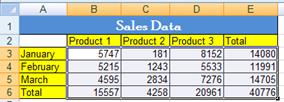
Figure 213
11. Hold Ctrl
and tap 1. Point to the Number tab. Select Accounting with no dollar sign,
click OK (Figure 214):
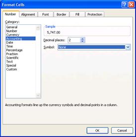
Figure 214
12. Highlight
A6:E6, Ctrl + 1, click the Borders tab. In the Line/Styles box, click the
medium thick line (second column, fifth down) (Figure 215):
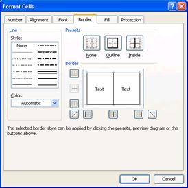
Figure 215
13. Click
the down arrow under color and select a color (Figure 216):
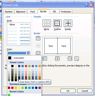
Figure 216
14. Click
the top line in the Border area (“Preview Diagram” area) (Figure 217):
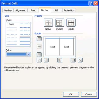
Figure 217
15. The most
important point that you must memorize to get this tab to work is this: ORDER
MATTERS – you must click Line/Style FIRST, Color SECOND, and then draw your
line in the Border area THIRD!
16. Now, use
the method just discussed to add a Dark Blue Double line to the bottom border
of our highlighted range (Figure 218):

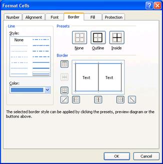
Figure 218
17. Click OK,
You should see (Figure 219):
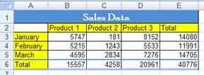
Figure 219
18. Now that we
have seen how to apply formatting, we need to look at how formatting can sometimes
trick us. If we are to become efficient with Excel we need to be able to match the proper formatting with what
actually sits in the cell!
Cell Number Formatting is the façade that sits on top of
data and formulas. What you see is not always what sits in the cell. For
example:
1. If
you see 3.00%, Excel more than likely sees 0.03
2. If
you see $56.70, Excel may see 56.695
3. If
you see 07/26/2005, Excel more than likely sees 38559
4. If
you see 9:30 AM, Excel more than likely sees 0.395833333333333
Let’s look at an example è
Here are the steps to
learn how to distinguish between Number Formatting and actual cell content!!!!
19. Navigate to
the sheet named “Formatting (3)”. You should see what is in (Figure 220). Read the labels in column A and type in
the number in column B. Column C tells you what is actually in the cell. The
key strokes for typing the numbers in are as follows:
i.
B2 è 1, 3, :, 3, 9, Ctrl + Enter (that is to say: Type
the number one, the number three, a colon, the number three, the number nine,
and then hold Ctrl and then tap Enter)
1. Each
time you hit Ctrl + Enter, look at what you see in the cell and compare that to
what you see in the formula bar
ii.
B3 è 1, 0, /, 2, 5, /, 2, 0, 0, 5, Ctrl + Enter
iii.
B4 è 1, 0, Ctrl + Enter (Notice that you did not have to
type in the dollar sign – the cell is preformatted)
iv.
B5 è 1, 0, Ctrl + Enter
v.
B6 è 3, Ctrl + Enter
vi.
B7 è 768, Ctrl + Enter
vii.
B8 è 768, Ctrl + Enter
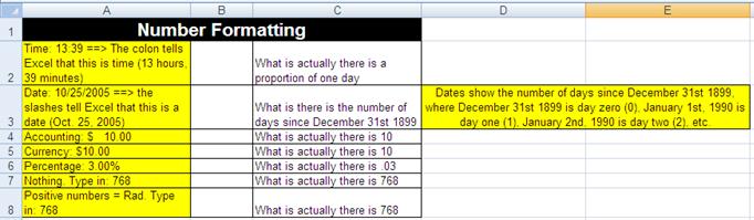
Figure 220
20. When you
are done you should see this (Figure 221):
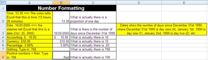
Figure 221: Notice that although we see the
word “Rad”, the formula bar shows us that the number 768 actually sits in the
cell.
21. The
keyboard shortcut to see the worksheet in “formula view” is Ctrl + ~ (The ~ key
is to the left of the “1” key and above the Tab key). Formula view shows you
what is actually in the cells, whether it is data, formulas. Hold Ctrl and tap
~ key (Figure 222):
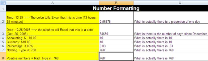
Figure 222
22. What you
see in Figure 221 is the façade. What you
see in Figure 222 is what actually is in
the cells. In addition, what is actually there in the cell is what Excel will
use for any formulas (whether calculating, text or other formulas).
23. Ctrl + ~ to
remove formula view (Ctrl + ~ is a toggle that switches between Formula view
and Normal view). Then click on each cell in column B and using the Format
Cells dialog box look at what Number format each cell is using
For Example in Figure 223
you can see that B2 has a time format
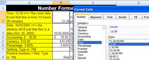
Figure 223
ii.
In Figure 224 you
can see the custom format (Custom formatting is not a topic that is book
addresses):
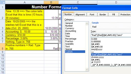
Figure 224
Rule #19: Cell Formatting is the façade that sits on top of
data and formulas. What you see is not always what sits in the cell.
The next page reminds you that there are six tabs in the
Formatting Cells dialog box. Two pages ahead we have an example of the
formatting façade getting in the way of accurate calculations!
Make a note that there are six tabs in the Format Cells
dialog box as seen below (Figure 225):
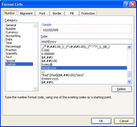
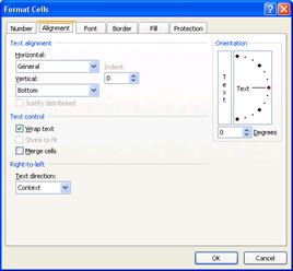
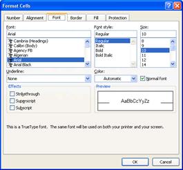
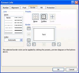
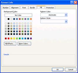
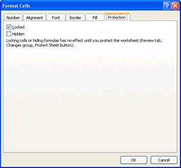
Figure 225
Here are the steps to
learn how to use the ROUND Function in Excel to insure accurate payroll
calculations when rounding to the penny is required
1)
Navigate to the sheet named “Round for Deduction”.
Before you make any calculations on this sheet, follow the calculations in step
2 and make the deduction calculations by hand with a pencil.
2)
How to use a formula to calculate a tax deduction
1.
Figure 226 shows
the Taxable earnings and short description of how to calculate a deduction. Use
Figure 227 to make a calculation by hand
using a pencil, an eraser and the rules of rounding to a penny!
Figure 226
Figure 227
3)
Now we can try it in Excel
4)
How to use a formula to calculate a tax deduction
1.
Before we create a formula to calculate the deduction,
let’s look at the Accounting Number format already applied in the cell range
B2:B4. Highlight the range and hold the Ctrl key, then tap the 1 key. You will
see the Format Cells dialog box (Figure 228):
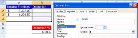
Figure 228
2.
To begin a formula, type the equal sign (Figure 229):
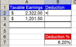
Figure 229
3.
With the thick white cross cursor, click on cell A2
(The cell reference A2 will appear in the formula) (Figure 230):
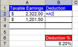
Figure 230
4.
Type the multiplication symbol (Figure 231):
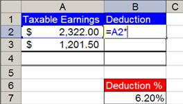
Figure 231
5.
Click on the cell with the deduction % as seen below (Figure
232):
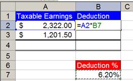
Figure 232
6.
Click the F4 key twice to lock the percent (Figure 233):
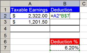
Figure 233
7.
Hold the Ctrl key, then tap the Enter key to place the
formula in the cell (Notice that you can still see the formula in the formula
bar (Figure 234):
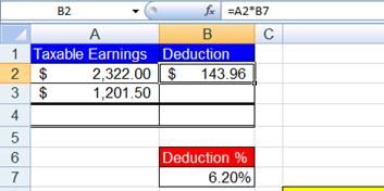
Figure 234
8.
Point to the fill handle (Little black box in lower
right corner of highlighted cell) (Figure 235):


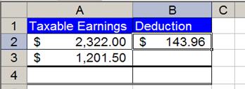
Figure 235
9.
With fill handle selected, copy formula from B2 to B3 (Figure
236):
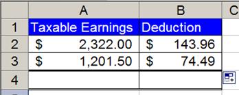
Figure 236
10. In
cell B4 add a SUM function by holding the Alt key and tapping the equal sign.
Verify that the SUM function selected the correct cells (Figure 237):
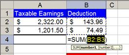
Figure 237
11. Hold
Ctrl and tap Enter (Figure 238):
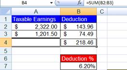
Figure 238
12. Go
down to the area with the yellow instructions and verify that you entered the
correct formula to calculate your payroll deductions. In cells E9 and E10 type
what you see in cells B2 and B3, respectively (DO NOT USE CELL REFERENCES). Create
a SUM function in cell E11 that adds the two cells above. (Figure 239):
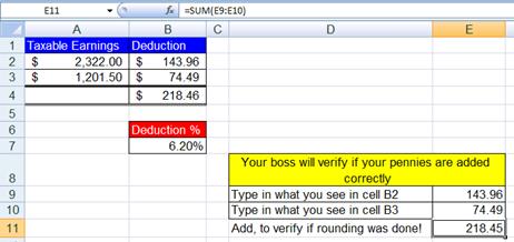
Figure 239
13.
Question: What is the problem here???!!?
14.
Answer: Excel did its part perfectly, but we did not!
We forgot to make sure that the formatting and the calculating formulas are
doing the same thing! To see how these are different, select the cell range B2:B4
and increase the decimals to three places. The Accounting Number format was only allowing us to see two decimals, but
what was actually in the cells was more than just two decimals. You should see
this after you increased the decimals to three places (Figure 240):
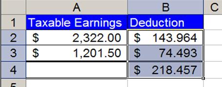
Figure 240
15. What
has happened here? The formulas underneath have calculated without rounding,
but the formatting on top has made it appear as if it has been rounded. The SUM
function does not look at formatted numbers, but instead looks at the unrounded
numbers.
16. The
solution is to make the format and the calculated numbers exactly the same by
using the ROUND function.
17. Decrease
the decimals to two places to restore the format to its original state. You
should see this (Figure 241):
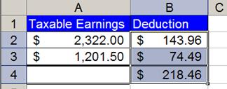
Figure 241
18. Add
a ROUND function to our formula by clicking in cell B2. To edit the formula
click the F2 keyboard button. You will see this (Figure 242):
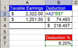
Figure 242
19. With
your cursor point in between the equal sign and the letter “A” and click to
insert your cursor into the formula. Then type the letters and characters
“ROUND(“ as seen here (Figure 243):
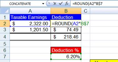
Figure 243
20. Then
point your cursor to the formula bar and click at the end of the formula as
seen here (Figure 244):

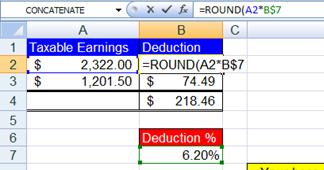
Figure 244
21. Type
the characters and numbers: “,2)” as seen here (Figure 245):
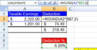
Figure 245
22. Hold
the Ctrl key and then tap the Enter key. Then copy the formula to cell B3. Now
you are done and you should see this (Figure 246):
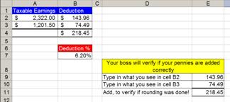
Figure 246
5)
Conclusions: because formatting (such as currency)
is like a façade that sits on top of the number, when you have a formula that
has the potential to yield more decimal places than the format displays, use
the ROUND function.
1.
For a payroll calculation that must be rounded to the
penny, instead of =A2*B$7, use =ROUND(A2*B$7,2); where the second argument “2” means round to the second
decimal.
2 means round to the penny (Payroll)
0 means round to the dollar (Income Taxes)
-3 means round to the thousands position. (Financial
Statements)
Rule #20:
Because formatting (such as currency) is like a façade that sits on top of the
number, when you have a formula that has the potential to yield more decimal
places than the format displays, use the ROUND function.
Next we will look at how to work with Date formatting.
With Date number format, dates
show the number of days since December 31st 1899, where December 31st 1899 is
day zero (0), January 1st, 1990 is day one (1), January 2nd, 1990 is day two
(2), etc. For example: January 1, 1900 is represented by the serial number 1;
January 2, 1900 is represented by the serial number 2; and April 23, 2006 is
represented by the serial number 38,830.
Here are the steps to
learn how to understand the Date number format and to make date calculations
(Excel date math)
1. Navigate
to the sheet named “Date Math”. You should see this (Figure 247):
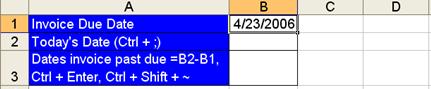
Figure 247
2. Hold
Ctrl and tap on the ~ key (this reveals what is actually in the cell; this is
called formula view). You should see what is in Figure 248. Understanding the Date format requires that you know that when
you type “4/23/2006” (Figure 247), Excel
sees 38830 (Figure 248). The “4/23/2006”
is the façade that we see. The 38830 is the serial number that Excel sees. This
serial number is very useful for making date calculations…
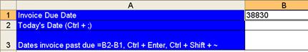
Figure 248
3. Hold
Ctrl and tap on the ~ key to remove formula view
4. Select
cell B2, Hold Ctrl and tap ; (semi colon) to put Today’s
date in the cell (Figure 249).
(Don’t worry if your day is different).
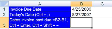
Figure 249
5. Select
cell B3, enter the formula “=B2-B1”, then hold Ctrl and tap Enter (Figure 250):
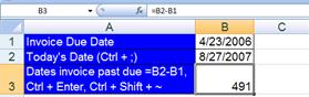
Figure 250
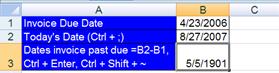
Figure 251
6. If
you see the formula result of 491 days (Figure 250), everything is working fine
and accurate.
7. But
if you see a formula result that is date formatted (Figure 251) You must be asking yourself What is going
on here? Why is there a date in our cell instead of the number of days the invoice
is past due? The answer is this: When you create a formula sometimes it brings
the format from the cells that you have referenced to the cell you are creating
a formula within.
8. To bring the format back to the “General format, Hold Ctrl
and Shift and tap ~ (Figure 252):
Figure 252
9. Figure
252 reveals the beauty of the serial
numbers that lie behind every date: it is easy to do date math! Whether you are
calculating an overdue invoice, your own age, or an estimate of the number of
days to complete a job, date math is amazing!
10. One final
note about Date format: Click in cell D1 and type the number 38830, then hold
Ctrl and tap Enter (Figure 253):
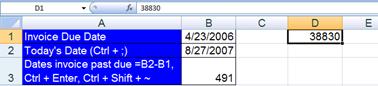
Figure 253
11. Hold Ctrl
and tap 1, click on the Number tab, click on Date (Figure 254):
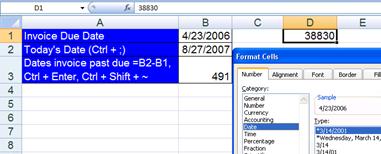
Figure 254
12. Click OK. Figure
255 illustrates directly that the number
38830 has a façade on top of it for us Excel users to see. In this way, we
understand that it is a date when we see it, but hidden underneath, Excel sees
the serial number so it can make date calculations!
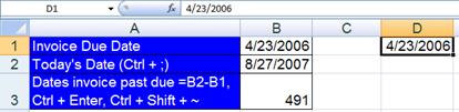
Figure 255
13. For
everyday Excel use, you can enter dates such as 4/23/2006, by typing the
numbers and forward slashes – Excel automatically enters the serial number
behind the scenes.
Rule #21: With
Date number format, Excel sees the number of days since December 31st 1899 (or January
1, 1900 (inclusive)). This allows us to make date math calculations.
Now that we have studied the Date number format façade and
how to use it, we can look at the Time number format façade and how to use it.
With Time number format, Excel
sees the proportion of one 24 hour day. For example: 8:00AM is represented by
the decimal number (also known as serial number or time value) 0.333333333333333;
6:21AM is represented by the decimal number .264583333333333; and 5:15:15 PM is
represented by the decimal number .718923611111111.
Here are the steps to
learn how to understand the Time number format and how to make time calculations
(Excel time math)
1. Navigate
to the sheet named “Time Formatting (1)”. You should see this (Figure 256):

Figure 256
2. When
entering times into Excl, you can use the following conventions (Figure 257):
Figure 257
3. Click
in cell A1 and type: 8, :, 0, 0, (space), A, M (said another way: type 8:00 AM).
Click in cell B1 and type 6:21 AM. Click in cell C1 and type 5:15:15 PM (Figure
258).

Figure 258
4. Hold
Ctrl and then tap ~ to see what Excel sees (Figure 259):

Figure 259
5. In
Figure 259, notice that the decimal
number that represents 5:15:15 PM is greater than the decimal value that
represents 8:00 AM. This insight will allow us to subtract the earlier time from
the later time and get the proportion of one day that has elapsed between the
two times.
6. Hold
Ctrl and then tap ~ to return to our normal view. In order to see that 8 hours
does represent .333 or 1/3 of a 24 hour day, click in cell D3 and type the formula
“two cells above divided by one cell above” (Figure 260):

Figure 260
7. Hold
Ctrl and then tap enter. Point to the fill handle and drag the formula from
cell D3 through F3 (Figure 261):
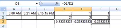
Figure 261
8. Highlight
the cells D3:E3, hold Ctrl and then tap 1, click on the number tab, click on
the Time category (Figure 262):
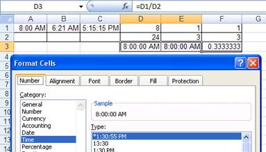
Figure 262
9. Click
OK. In Figure 263, we can see that 8/24
or 1/3 is .333333333333333, but when we apply a Time format, the Excel user
sees 8:00 AM.

Figure 263
10. As an extra
bonus, click in cell F3 and apply the Fraction format. After you apply this
format you should see this (Figure 264):
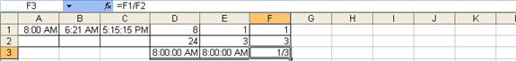
Figure 264
11. With our
new understanding of the Time format, we would like to make some time
calculations in Excel.
12. Navigate to
the sheet tab named “Time Formatting (2)” You should see this (Figure 265):
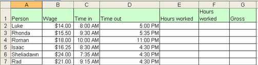
Figure 265
13. We would
like to use Excel to keep track of employees work hours and gross pay. Click in
cell E2 and subtract the earlier time from the later time (“one to my left
minus two to my left”) (Figure 266):
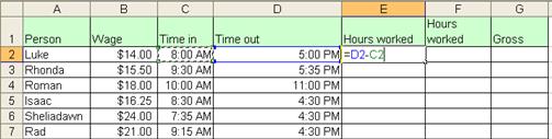
Figure 266
14. Hold Ctrl
and then tap Enter (Figure 267). We see
is Figure 267 that the Time format has
carried forward into our cell with the formula.
Figure 267
15. Hold Ctrl
and Shift and tap ~. In(Figure
268).
we see the proportion of the day that Luke has worked.
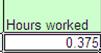
Figure 268
16. Hold Ctrl
and tap 1, select the Number tab, click on the Time category, click on the
second time type in the list (Figure 269):
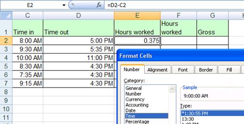
Figure 269
17. Click in G2
and type the formula as seen in Figure 270:
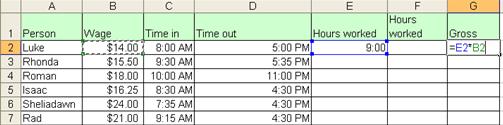
Figure 270
18. Hold
Ctrl and tap Enter. What is wrong with Figure 271?
Nothing! If WE were trying to multiply 9 hours times $14.00, we did not
accomplish this. We made the wrong calculation. Excel did not make the wrong
calculation. The resultant answer, 5.25, is exactly what we asked Excel to
calculate, namely: 0.375*14.
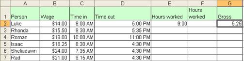
Figure 271
19. Delete the
contents of cell G2. In cell F2 type the formula “=(D2-C2)*24” (Figure 272). Notice that we had to know our order of
operations (the subtraction is in parenthesis) and we had to know that 24 is a
number that will not vary (thus it is OK to type into our formula).
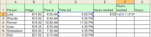
Figure 272
20. Hit Tab.
Type the formula “one to my left times four to my left” in cell G2, and then
hold Ctrl and tap Enter. Then Hold Ctrl and Shift and
tap the $ key (this is the keyboard shortcut for the Currency format). You
should see this (Figure 273):
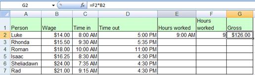
Figure 273
21. Highlight
the range E2:G2, point to the fill handle and with your angry rabbit, double
click the fill handle to copy the formulas down (Figure 274):
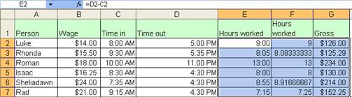
Figure 274
22. With our
knowledge of the Time format, order of operations and non-varying numbers, we
have created formulas that we can use for timesheet calculations.
Rule #22: With
Time number format, Excel sees the proportion of one 24 hour day. This allows
us to make time math calculations.
Next
we will turn our attention to Excel’s Charting capabilities.
Charts
Charts and graphs are a means to visually articulation
numerical data. There are times when a picture (chart or graph) tells a
thousand words. Charts and graphs can deliver a message in a more immediate
way. Although a chart or graph lacks the detail of all the numbers, it quickly
articulates its message in an effective way.
Navigate to the sheet tab named “Charts (1)”.
In Excel, after highlighting your numerical data and labels,
you can initiate chart creation from the Chart Group on the Insert Ribbon. (Figure
275):

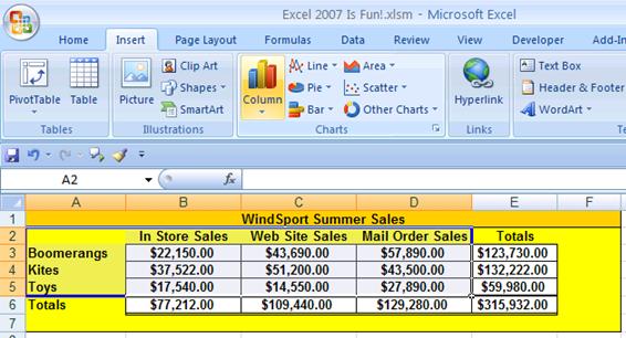
Figure 275
After you initially create your Chart from the Chart Group on
the Insert Ribbon, you can use the three Context-Sensitive Ribbons for Charts
or you can right-click the different elements of the Chart. (Figure 276):
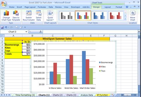
Figure 276
In Figure 276 we can
see a “Column” chart type. However, there are many charts to choose from and
choosing the correct one can sometimes be tricky. We will look at two chart
types: Pie chart and a Column chart with multiple series data. If you would
like to learn about more of the built in chart types, Click F1 (Microsoft Help)
and type “Available chart types”. There is an article that gives an excellent
example of each chart type.
Here are the steps for
creating a Pie chart
1. Navigate
to the sheet named “Charts (1)”. You should see this (Figure 277):
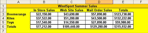
Figure 277
2. In
Figure 277 we can see that WindSports
Sales are broken apart into categories. Vertically, in Column A, we can see
that WindSport has categorized the sales according to the products that they
sell: boomerangs, kites and toys. Horizontally, in Row 2, we can see that
WindSport has categorized the sales according to the sales channels that they
use for selling: In Store, Web Site and Mail Order. In addition, they have
listed totals for each category and an overall total in the lower-right corner.
3.
For our first Chart we would like to show how each
product total contributes to the overall total. This means that we are
comparing three “parts” (boomerangs, kites, toys) to the overall total to see
what proportion or percentage that each contributes to the whole. Anytime you
have this situation (comparing parts to the overall total), a Pie chart type is
an excellent choice.
4.
Highlight the range A3:A5, Hold Ctrl, Select the range
E3:E5 (you are selecting two ranges of cells that are not adjacent to each
other), and then point to the Pie chart icon button in the Charts Group on the
Insert Ribbon (Figure 278).
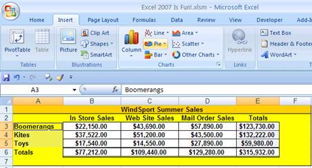
Figure 278
5. Click
on the Pie chart icon button and then point to the first option. As you can see
in (Figure
279).,
Excel gives you a description of what the chart should be used for. As you
learn how to make charts, you can read these as you are trying to decide which
chart is best for your message.
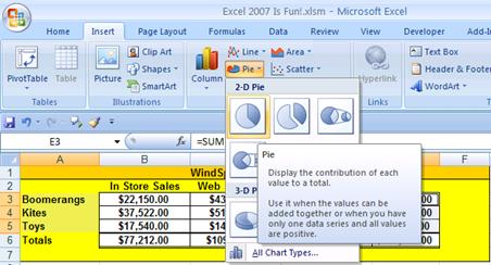
Figure 279
6. Click
on this first option to create your Pie chart. In Figure 280 you can see that it placed a pie chart on
top of the worksheet and opened the three context-sensitive Ribbons for charts.

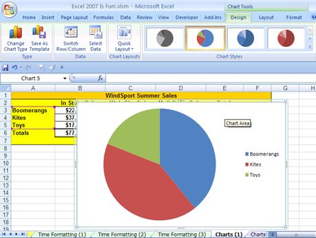
Context-Sensitive Ribbons
|
|

 Figure 280
7. To
change the size of the chart, hold the Shift Key and point to the upper left corner
of the chart and when you see a diagonally pointing black arrow, click and drag
inward. You should change the size to about the same size as seen in Figure 281:
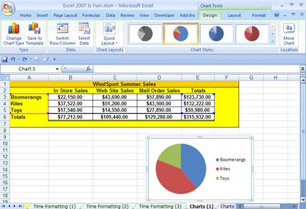
Figure 281
8. Click
on the “Quick Layout” icon button on the Chart Tools Design Ribbon and point to
the “Layout 1” option (Figure 282):
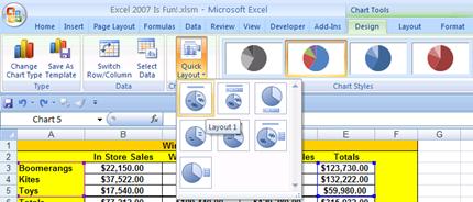
Figure 282:
9. In
Figure 283 you should see that the Quick
Layout added a Chart Title, and the category names with percentages that convey
how much each part contributes to the whole.
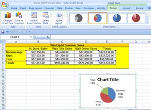
Figure 283
10.
Click on the “See More Selections” Arrow in the Chart
Styles Group (Figure 284):

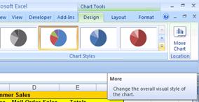
Figure 284
11.
After you click on the “See More Selections” Arrow,
choose “Style 10” as seen in Figure 285:
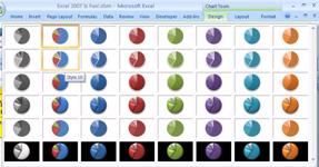
Figure 285
12.
After clicking on Style 10 you should see this (Figure 286):
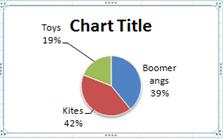
Figure 286
13.
Now we need to Change the Chart Title. Click once on
the Chart Title, then click a second time so that an I-beam cursor is flashing
in the Chart Title(Figure 287):
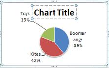
Figure 287
14.
Hold Ctrl and tap the “A” key
(keyboard shortcut for Select All)
(Figure 288):
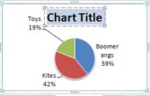
Figure 288
15.
Type “Summer Sales.” And then click on the outer edge
of the Chart to register the “Summer Sales” Title. (Figure 289):
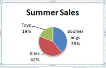
Figure 289
16.
To change the size of the chart, hold the Shift Key and
point to the upper left corner of the chart and when you see a diagonally
pointing black arrow, click and drag outward. You should change the size to
about the same size as seen in Figure 290:
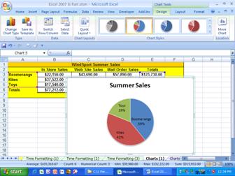
Figure 290
17.
To move that chart to below the Sales Table, Hold Ctrl and Click on the Chart (This selects the chart so
that you can move it). Then click and drag your Pie chart as seen in Figure
291. Then Hold Ctrl and tap the F1 key to
hide the Ribbons.
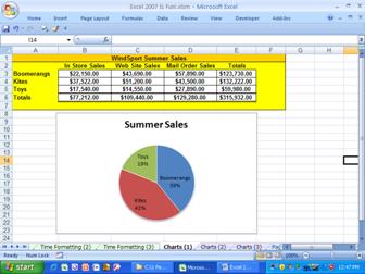
Figure 291
18.
In Figure 291 we
can see that we have created an appropriate chart that shows how much each
product contributed to the overall total sales. We can clearly see that the Toy
products contribution the smallest amount to the overall total as compared to
the other two products.
19.
For our next chart, Navigate to the sheet tab named
“Charts (2)”.
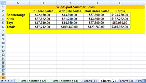
Figure 292
Here are the steps for
creating a Column chart with multiple series data
20.
The first Pie chart we made showed the product
categories, but we only looked at the totals. Next we would like see how each
of the three product categories compares in each sales channel. Now we could
make three different Pie charts, but there is a better way than that. If we use
a Column chart we can see the three products compared across the sales channel
categories (Column chart with multiple series data). In Figure 292 we can see that there are three product
categories and each one of those categories has a sales number for each sales
channel. For example, for Toys we have the numbers $17,540.00, $14,550.00, $27,890.00.
These three numbers are called a “data series” in Excel. There is a data series
for each product and a data series for each sales channel. For example, the
data series for the In Store sales channel would be $22,150.00, $37,522.00,
$17,540.00.
21.
Highlight the range A1:D5 and click on the Column icon
button in the Chart Group on the Insert Ribbon (Figure 293).
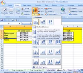
 Figure 293
22.
As seen in Figure 293,
click on the first option in the drop-down icon list named “Clustered Column”
The result can bee seen in Figure 294:


Figure 294
23.
An excellent aspect of this chart is that you can
quickly change the orientation of a Clustered Column chart by clicking on the
Switch Rows/Columns icon button in the Data Group on the Chart Tools Design
Ribbon. Figure 294 shows the icon button
to click. Figure 295 shows the “switched”
Chart.
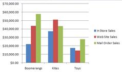
Figure 295
24.
Click the Switch Rows/Columns icon button again to
switch back. Then click on the Charts Tools Layout Ribbon (Figure 296):
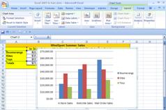
Figure 296
25.
As seen in Figure 296,
the Layout Ribbon has many chart elements that you can add. Let’s add a Chart
Title. Click on the Chart Title icon button in the Labels Group on the Chart
Tools Layout Ribbon. Then as seem in Figure 297,
click on the “Above Chart” item on the icon drop-down list.
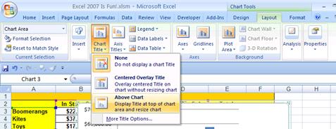
Figure 297
26.
When the Chart Title appears, highlight the words and
type “Product Sales for Each Sales
Channel” (Figure 298):
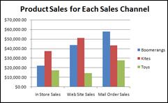
Figure 298
27.
As seen in Figure 299,
we next want to click on the Chart Tools Format Ribbon. The Chart Tools Format
Ribbon allows you to format any of the chart elements after you have selected
the element that you want to format. An alternative to using this Ribbon is to
select the Chart Element and then right-click the element. Let’s try this.
Click on the vertical axis (also known as the y-axis). When you click on the
vertical axis, a thin black outline will appear that let’s you know that you
have selected it (Figure 300).
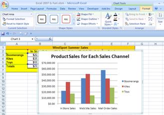
Figure 299
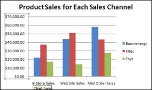
Figure 300
28.
Once you have the element selected that
you want to format, use the keyboard shortcut for the Formatting
Chart Element dialog box =: Ctrl + 1 (Figure 301):
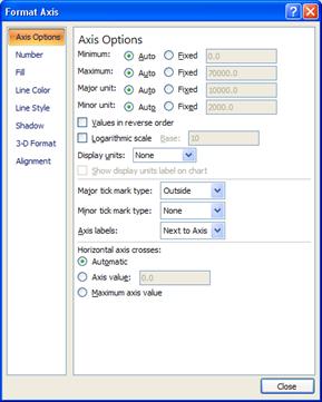
Figure 301
29.
On the Left side of the Format Axis dialog box, click
on “Number”. Make sure that the Currency Number format is selected, change the
decimals to 0, and click Close (Figure 302):

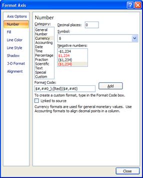
 Figure 302
30.
The Chart should
look like this (Figure 303):
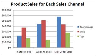
Figure 303
31.
In Figure 303 we
can see how each of the three product categories compares in each sales
channel. The smallest sales for a product are the sales for Toys sold through
the web site.
In our nest section, we want to talk about Page Setup.
Navigate to the sheet tab names “Page Setup”.
Page Setup
To see how Page Setup works, click on the “Page Layout”
Ribbon. In Figure 304 you can see that
there is a Payroll sheet. Imagine that your boss asked you to print out this
report. To see what it would look like before you print it out, click on the
Orb.

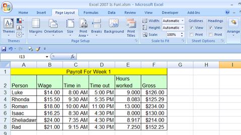
Figure 304
After you click on the Orb, point to the Print icon and then
to the Print Preview icon. Notice in Figure 305
that a screen tip pops up and let’s us know that there is a faster way to see
Print Preview: the keyboard shortcut for Print Preview is Ctrl + F2. Click the
Esc key (upper left corner) twice. Then use you newly discovered keyboard
shortcut Ctrl + F2 to open up Print Preview.
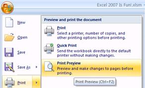
Figure 305
Ctrl + F2 opens up Print Preview. As we can see from Figure 306, the sheet will print out in the upper left
corner. This does not look like a professional payroll report. We need to fix
it! Click the Esc key to get back to Normal View.
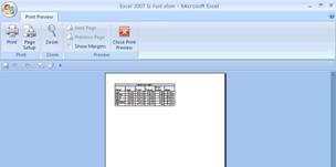
Figure 306
Here are the steps for
setting up your sheet for printing
1.
After you click the Esc key you are back in Normal
view. As seen in Figure 307, click on the
Page Setup Dialog Launcher in the lower right corner of the Page Setup Group on
the Page Layout Ribbon.
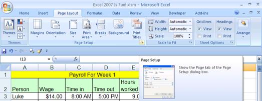
Figure 307
2.
After you click the Page Setup Dialog Launcher, you
should see this (Figure 308):

Figure 308
3.
The advantage of using the Page Setup dialog box is
that you do not need to keep going up to the Ribbon to launch the dialog box.
For example, click on the “Sheet tab” (as seen in Figure 309) that contains two parts in the Ribbon all
in one dialog box. As seen in Figure 310,
the Print Titles icon button in the Page Setup Group on the Page Layout Ribbon
launches the Page Setup dialog box with the Sheet tab showing. As seen in Figure
311, the Sheets Options Dialog Launcher
on the Page Layout Ribbon launches the Page Setup dialog box with the Sheet tab
showing also. However, with all this said about the advantages of the Page
Setup dialog box, the reason Microsoft allows users different options for the
various elements in Excel is because users have different preferences. So
ultimately you get to decide which method you like better. However, in the
long-run, it is not disputed that the fastest and most efficient way to
accomplish things is Excel is to use as many keyboard shortcuts as possible.

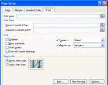
Figure 309

Figure 310

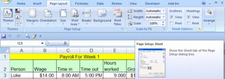
Figure 311
4.
Click the Esc key. Then use the keyboard shortcut for Page Setup: Alt + P + S + P (Tap each
key in succession). You should see the Page Setup dialog box. As seen in
Figure 312, click the dialog buttons for
Landscape and “Fit to: 1 page(s) wide by 1 tall.” This will orientate the
printed page in the same fashion as the Payroll table: wider than it is tall.
Also, the “Fit to: 1 page(s) wide by 1 tall.” will assure that if the Payroll
table is bigger than the page Excel will automatically shrink it to fit on one
page!
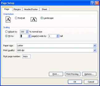
Figure 312
5.
Next, click on the Margins tab and then click the
Horizontal checkbox in the Center on page area as seen in Figure 313. This will center it on the page
horizontally for a professional look. Do you know what Margins do? Margins are
how far in from the edge of the paper the worksheet content can be printed. For
example, if we did not center the Payroll table, the left edge of the Payroll
table would be printed .7 inches from the left side of the piece of paper. Also
in Figure 313 you can see that you have
the option to change any of the page margins (left, right, top, and bottom) and
also you can change the location that Headers and Footers are printed. In Figure
313 you can see that the Headers and
Footers will be printed .3 inches from the top and bottom of the page. In our
next step we will add Headers and Footers.
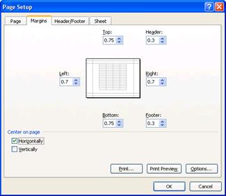
Figure 313
6.
As seen in Figure 314
click on the Header/Footer tab.


Button to build Custom Footers
|
|


Drop-down for built-in Footers
|
|
Button to build Custom Header
|
|
Drop-down for built-in Headers
|
|

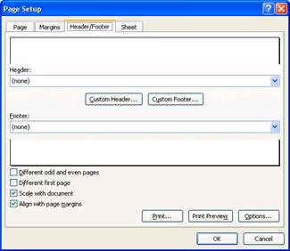
Figure 314
Note: there is a good
alternative for creating Headers and Footers. If you choose the Header &
Footer in the Text Group on the Insert Ribbon, you can create Headers and
Footers. (Keyboard shortcut for Headers and Footers is
Alt + N + H (this puts you into Page Layout View with the Headers enacted), and
the keyboard shortcut to get out of Page Layout View is Alt W + L (this puts
you back in Normal View). If you are only adding Headers and Footers
this is the better method. However, if you are adding many Page Setup elements
all at once, then the Page Setup dialog box is more efficient.
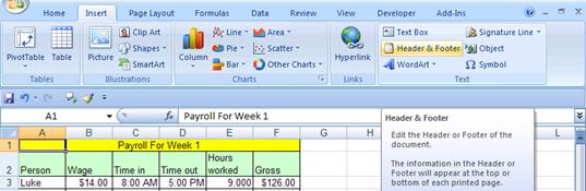
Figure 315
7.
While still viewing the Header/Footer tab in the Page
Setup dialog box, click the drop-down arrow for built-in Footers and select
“Page 1 of ?” as seen in Figure 316. This
is Excel Code that will automatically put the correct page numbers on each page
that prints out. (In our case we have only one page.)
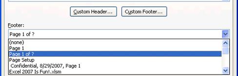
Figure 316
8.
Next, click on the Button to build Custom Headers. A
new dialog box pops up on top of the Page Setup dialog box (Figure 317):


Header dialog box is on top of the Page Setup dialog box
|
|
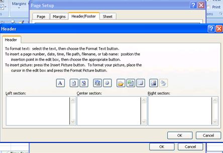
Figure 317
9.
As seen in Figure 318,
click in the left section and click on the Insert File Name (this inserts the
code that automatically puts the file name in your header – even if you change
the file name, your header will automatically update).
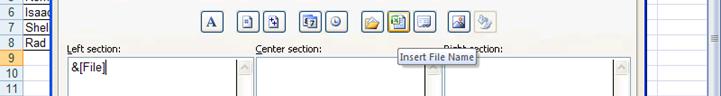

 Figure 318
10.
 As
seen in Figure 319, click in the center
section and click on the Insert Sheet Name (this inserts the code that
automatically puts the sheet name in your header – even if you change the sheet
name, your header will automatically update).
As
seen in Figure 319, click in the center
section and click on the Insert Sheet Name (this inserts the code that
automatically puts the sheet name in your header – even if you change the sheet
name, your header will automatically update).
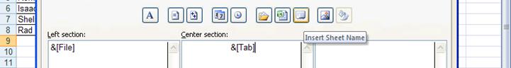
 Figure 319
11.
As seen in Figure 320,
click in the right section and click on the Insert Date (this inserts the code
that automatically puts today’s date in your header – if you print it out at a
later date, your header will automatically update).
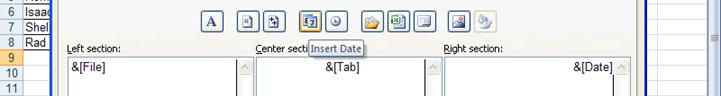

 Figure 320
12.
As seen in Figure 321,
click OK in the Header dialog box:

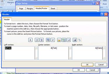
 Figure 321
13.
As seen in Figure 322Figure
321, click OK in the Page Setup dialog
box:

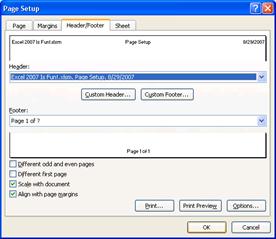
 Figure 322
14.
To
see a preview of your Page Setup before you print, Hold the Ctrl key and tap
the F2 key (Figure 323):
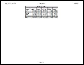
Figure 323
15.
The print preview that we see in Figure 323 is much better than the one we saw in Figure
306. Not only that, but with the ability
to do Page Setup, you will be the heroine or hero in many office setting
(because usually people can’t figure out how to print their sheet correctly!
16.
In our next section, we want to take about data
analysis topics such as sorting, subtotals and PivotTables.
The essential beauty of Excel is that you can make
calculations and analyze/manipulate data quickly and easily “on the fly!”
What-if analysis is easy in Excel. You can Sort to see which Sales Rep had the greatest
sales, create Subtotals by Region, and do complex data analysis such as
summarizing on multiple criteria (PivotTables). (This section is only a brief
look at Excel’s infinite Analyzing capabilities…). For this section we will
look at Sorting, Filtering, automatic Subtotals and a basic PivotTable.
The #1 MOST IMPORTANT THING TO REMEMBER WHEN YOU START TO
USE EXCEL’S DATA ANALYSIS TOOLS IS:
Rule #24: Before
you use Excel’s Data Analysis Tools: the data must be in proper Excel “List” or
“Table” Format. This format is as follows: 1) First row has field names with
formatting that is different from the rest of the data; 2) No blank field names;
3) Columns are called Fields; 4) Rows are called records; 5) No blank columns
(fields); 6) No blank rows (records); 7) Blank rows and columns and/or Excel’s
column headers (A, B…) and/or row headers (1, 2…) must separate the Excel List
from other data
Columns are called “Fields”. Fields are the variable data
for each record. Rows are called “Records”. Records are individual collections
of the fields. For example, navigate to the sheet tab named “Analyze Data”,
click on the Data Ribbon. You should see this (Figure 324): Note: your data
may not be in the same order as the picture.
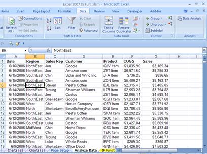
Figure 324
In Figure 324 we can
see:
1. Proper
Excel “List” or “Table” Format, which will refer to as “Excel’s List/Table
format” (this is because in Excel 2003 it was called “List” and in Excel 2007
it is called “Table”)
2. Each
row represents one Sales Transaction
i.
Each sales transaction is one new record
ii.
Each record is an individual collection of the seven
fields
3. The
first seven columns represent fields
i.
Each field is a variable
1. For
each new transaction it can have a different date or different region or
different sales rep, etc.
Steps to Sort on various
criteria
1.  The
method of sorting we will look at involves turning on the “Filter” with the keyboard shortcut for Filter: hold Ctrl and Shift, then tap
the “L” key. In Figure 325 you can
see that that keyboard short cut added drop-down arrows at the top of each
field and turned on the Filter button in the Sort and Filter Group on the Data
Ribbon.
The
method of sorting we will look at involves turning on the “Filter” with the keyboard shortcut for Filter: hold Ctrl and Shift, then tap
the “L” key. In Figure 325 you can
see that that keyboard short cut added drop-down arrows at the top of each
field and turned on the Filter button in the Sort and Filter Group on the Data
Ribbon.


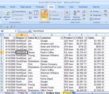
Figure 325
2. Point
to the drop-down arrow for the Sales
field and point to “Sort Largest to Smallest” (Figure 326):
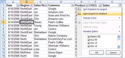
Figure 326
3. As
seen in Figure 327, instantly, the whole
table is sorted by the sales numbers in the Sales field. We can easily see that
Sales Rep Luke had the two largest sales.
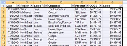
Figure 327
4.
Next click on the drop-down arrow for the Sales Rep
field and click on the “Sort A to Z” from the drop-down list (Figure 328)
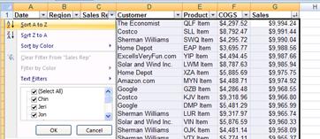
Figure 328
5. As
seen in Figure 329, instantly, the whole
table is sorted by the names in the Sales Rep field, with Chin at the top.
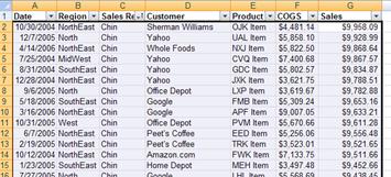
Figure 329
6.
To see how to sort without the Filter turned on, turn
off the Filter with the keyboard shortcut Ctrl + Shift + L, then click in cell
B6 (Figure 330):
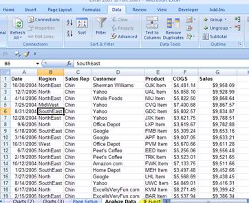

 Figure 330
7.
With only one cell selected in the Region field column,
click the “A è
Z” icon button in the Sort & Filter Group on the Data Ribbon (Figure 330)
8.
As seen in Figure 331,
the whole table was sorted by the region names in the Region field column.
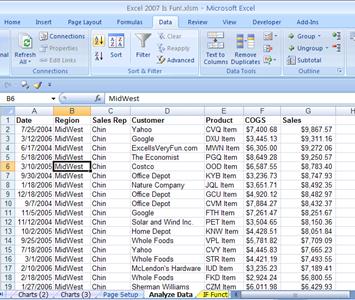
Figure 331
Rule #25: Before click the “A è Z” icon button in the Sort & Filter Group on the
Data Ribbon, make sure your block of data is in the Proper Excel List/Table
Format and highlight only one cell in the field you want to sort.
Steps to Filter your data
1. Navigate
to the sheet named “Filter”. You can use this keyboard shortcut to move down
two sheets: Hold Ctrl and then tap the Page Down key twice. You should see the
data as seen in Figure 332. Then, turn on
the Filter using the keyboard shortcut: Ctrl + Shift + L

Hold Ctrl and Shift at the
same time and then tap “L” to turn on the Filter
|
|
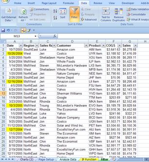
Figure 332
2.
To see the Sales that are Above Average, click the
drop-down arrow at the top of the Sales field and in the drop down list point
to Number Filters and then point and click on Above Average (Figure 333).
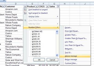
Figure 333
3.
As you can see in Figure 334 Excel quickly shows us the results. Notice two things: 1) the
drop-down arrow at the top of the Sales field contains a “Filter” icon to let
us know that the field has been filtered; 2) the row numbers are the color blue
to let you know that the rows with records that are not above average have been
hidden. For example, you can see in Figure 334
that rows 7, 8, 9, and 10 are hidden.

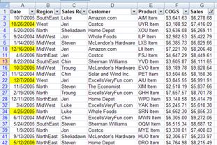
Figure 334
4.
To clear the filter, click on the drop-down arrow at
the top of the Sales field and click on the item “Clear Filter From Sales”.
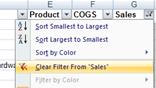
Figure 335
5.
To see a brief example of the options available for
filtering words, click on the drop-down arrow at the top of the Customers
fields and point to Text Filters (Figure 336).
Notice that you can uncheck any customers you would like if you only want to
see a selection of Customers. In addition, you can see the Text Filters
available.
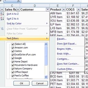
Figure 336
6.
Next we want to see how to sort by color. Notice in Figure
337 that the color yellow is added to
some of the dates. This color was to tag those records for auditing. Instead of
scrolling down and seeing each record one at a time, we can sort by color.
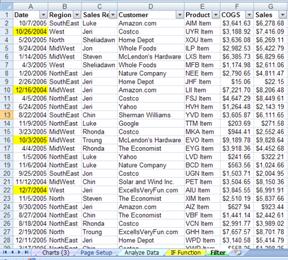
Figure 337
7.
Click on the drop-down arrow at the top of the Date
fields and point to Sort by Color and then click on the color yellow (Figure 338):
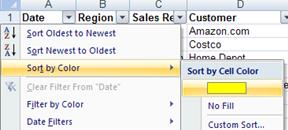
Figure 338
8.
In Figure 339 we
can see that very quickly our records that we need for auditing are sorted to
the top.
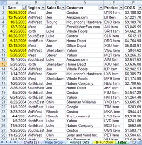
Figure 339
9.
As you can see to our brief introduction to Sorting and
Filtering, it allows us to do data analysis efficiently. In addition, you can
also see from some of the drop down menus that we only looked at a small
fraction of the possibilities!
10.
In our next section, we will look at another data
analysis tool: Subtotals.
Steps to add automatic
Subtotals
1. Before
we look at Subtotals, navigate back to the sheet tab named “Data Analysis” (Figure
341):

Figure 340
2.
Subtotals are one of the greatest tricks in Excel
because using the Subtotal feature quickly goes through the whole table and inserts
rows and adds totals for the column that you specify. In our case, we will be
able to very quickly add totals for all the regions and Sales Reps!
3.
An important point to make here is this: DON’T USE THE
SUBTOTALS FEATURE FOR A PARTICULAR FIELD UNTIL YOU HAVE SORTED THAT FIELD.
4.
We have already sorted the region and the Sales Rep
fields so that we can use the Subtotal feature.
5.
As seen in Figure 341,
click on the Subtotals icon button in the Outline Group on the Data Ribbon.
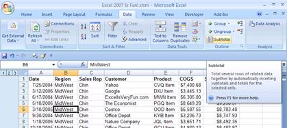
Figure 341
6. You
should see Subtotal dialog box as seen in Figure 342. . Notice that the whole table was highlighted when you invoked
the Subtotals dialog box (this is because you have your data in proper Excel List/Table
format). Using the drop-down arrow for the “At each change in” textbox, select
the Region field. For the “Use function:”, use the Sum function. For the “Add
subtotals to:” checkboxes check the Sales field.
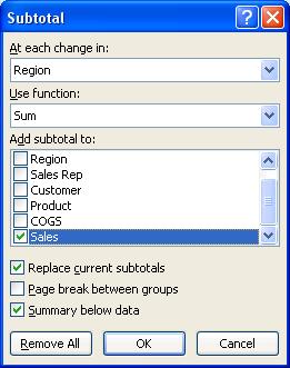


 Figure 342
7. Click
OK. You should see something similar to Figure 343.
On the left of your screen you should see three little blue-gray boxes with the
numbers 1, 2, and 3 in
them. These are called Outline buttons.

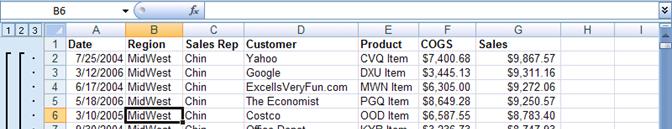
Figure 343
8. Click
the “2”
Outline button and you should see subtotals similar to those as seen in Figure 344. The plus and minus symbols are collapse
and expand symbols. You can use these to expose the data for a particular Region.
You can also use the “3”
Outline button to expose all the records. Before you click on the “3” Outline button, notice that
there are 200 rows of sales transaction data that the Subtotals feature
traversed in less than a second! This is an amazingly efficient feature in
Excel!
The Subtotal feature works through 200 rows of data
quickly
|
|

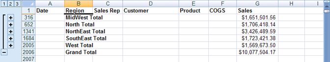
Figure 344
9. Click
on the “3”
Outline button to show all the records again (Figure 345):
Figure 345
10. Open the Subtotals dialog box with the keyboard shortcut:
Alt + A + B. As seen in Figure 346,
use the drop-down arrow next to the “At each change in” textbox to select the
Sales Rep field. For the “Use function:”, use the Sum function. For the “Add
subtotals to:” checkboxes check the Sales field. Finally (this is the most
important step when adding a second Subtotal), un-check the “Replace current
subtotals” checkbox and then click OK.
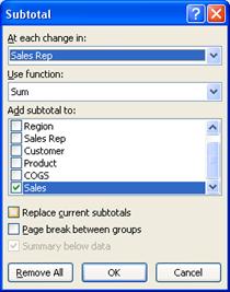
 Figure 346
11. As seen in Figure
347, a fourth Outline Level has been
added.

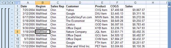
Figure 347
12. Click on
the “3”
Outline button. As seen in Figure 348,
Subtotals have been added for both the Region and Sales Rep fields. With this
Subtotal Data Analysis, we can easily pick how each Sales Rep did in each
Region.
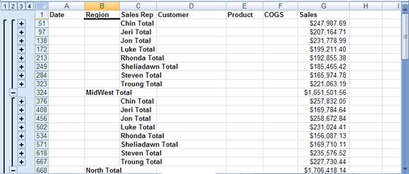
Figure 348
13. To get rid
of the Subtotals, use the keyboard shortcut to open the Subtotals dialog box:
Alt + A + B and then click the “Remove All” Button
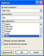
14.  In
our next section we will talk about the most powerful toll in Excel, the
PivotTable.
In
our next section we will talk about the most powerful toll in Excel, the
PivotTable.
Rule #27:
Before adding automatic Subtotals, sort your field. If you want to add a
Subtotal to a Subtotal, Be sure to uncheck the “Replace current subtotals” check box.
Steps to create a basic
PivotTable
1. What
is a PivotTable? It is a quick way to analyze data such as summing up data in a
rectangular table shape when you have more than one category to summarize upon.
Figure 349 shows us an example of what
would like to accomplish from our data. As you can see we have two categories
(Sales Rep and Region) and we have a rectangular table shape. To create this
without using the PivotTable feature, but instead to use functions, would be
very time consuming.
Figure 349
2. To
create something similar to what we see in Figure 349, make sure you have one cell in your data table selected and
that your data is in proper Excel List/Table format, then click on the
PivotTable icon button in the Table group on the Insert Ribbon (Figure 350):
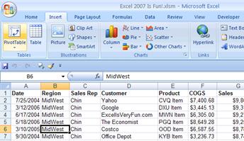
 Figure 350
3. Notice
that because we are using proper Excel List/Table format and we had selected
one cell in the middle of our data, all the data was automatically selected. As
we can see in Figure 351 Create
PivotTable dialog box opens and we can see that the range A1:G2000 is selected.
In addition, we want to create our PivotTable on a new sheet and so we will
accept the defaults and then click the OK button.
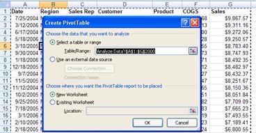
Figure 351
4.
In Figure 352 we
can see that the PivotTable Field List Task Pane pops up and a new sheet is
added to the workbook. All we have to do in order to create a table with the
two categories Sales Rep and Region is to click on the checkboxes for those two
fields (after all this is just field list).

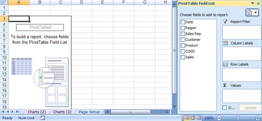
Figure 352
5.
As seen in Figure 353,
by checking the two fields, both were added as Row Labels.


Click on the Region field and drag it to the Column
Labels’ area
|
|

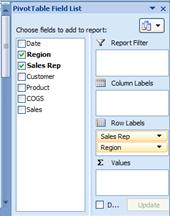
Figure 353
6.
As seen in Figure 353,
because we want the Sales Rep field as a Row Label and our Region as a Column
Label, we will click on the Region field in the Row Labels’ area, hold the
click, and drag it to the Column Labels’ area
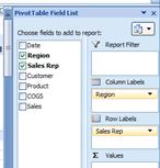
Figure 354
7.
As seen in Figure 354, we have our two category
labels
8.
As seen in Figure 355,
we can see our PivotTable taking shape. We can see that the Sales Rep labels
and the Region labels in our worksheet. We can see that two context-sensitive
Ribbons for the PivotTable have appeared (PivotTable Tools Options and Design
Ribbons).


We can see that two context-sensitive Ribbons for the PivotTable
have appeared.
|
|


We can see that the Sales Rep labels and the Region labels in our
worksheet.
|
|
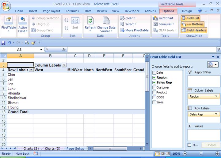
Figure 355
9.
Because we cannot see the whole PivotTable, Zoom slider
in the Status Bar to move down to 90% view. As seen in Figure 356, click the “Zoom Out button (minus sign) to
move to 90% view.
Figure 356
10.
As seen in Figure 357,
we can now see the whole PivotTable.
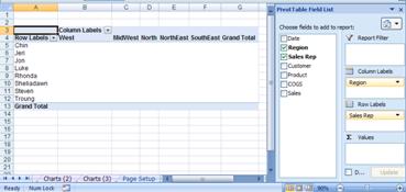
Figure 357
11.
Next, as seen in Figure 358,
click on the Sales field in the PivotTable Field List Task Pane – this adds the
Sales field to the Values area. PivotTables use the Sum Function by default,
which is what we wanted in our case. To see how to change the function and to
format the Sales numbers, click the close “x” button in the top right corner of
the PivotTable Field List Task Pane and then click in cell A3.

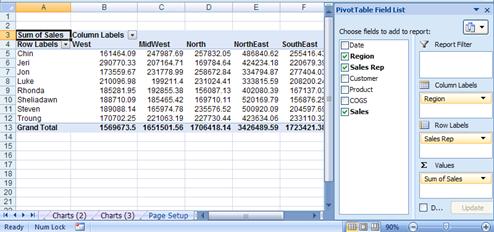
Figure 358
12.
With your cursor in cell A3, right-click and point to
“Value Field Settings” (Figure 359):
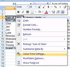
Figure 359
13.
As seen in Figure 360,
the Value Field Settings dialog box should appear: If you were to change the
function, you could do so in the “Summarize value field by” function list.
Because we want to change the Number formatting, we will click the Number
Format button.


If you were to change the function, you could do so in
the “Summarize value field by” function list.
|
|
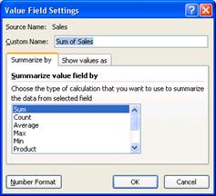
Figure 360
14.
This is another one of those situations when two dialog
boxes are opened. When the Format Cells dialog box appears, select the Currency
Number format. Then click the OK button on the Format Cells dialog box. Then
click the OK button on the Value Field Settings dialog box. (Figure 361):
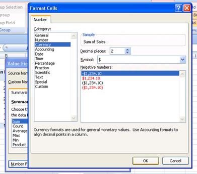
Figure 361
15.
With only a few clicks, the PivotTable is done. Even
better than with Subtotals, we can easily see how each Sales Rep did in each
Region (Figure 362):
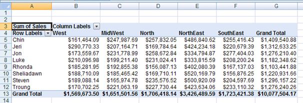
Figure 362
Rule #28:
When your data is in Proper Excel List Format, PivotTables are the most
powerful tool in Excel. Don’t be afraid of them, there are just tables with
variables on the left (Row) and top (Column) side and an intersecting
calculation in the middle (such as summing)!
In this next section we will talk about a built-in Excel
function called the IF function. The IF function is great for when you need to
put one of two things into a cell. For example, when you are calculating whether
or not you get a bonus at work, you would say something like, “If I make sales over or equal to $5,000, I
get a $100 bonus, otherwise I get no bonus.” Notice that the words that we
use to describe whether or not we get a bonus start with the word “If”! This is
why Excel named the function “IF”.
In our case the logical test would be: “Sales >=$5,000” (in words: “If I make sales over or equal to
$5,000”). This logical test will either be TRUE or FALSE. If the logical test
is TRUE, then we get our bonus of $100. If the logical test is FALSE, then we get a bonus of $0 (we did not exceed or equal the
sales hurdle of $5,000).
The built-in Excel IF function will automatically tell you
whether or not you earned a bonus! All you have to do is tell the IF function three things:
- What
the logical test is
- What
the bonus amount is (Value to put in the cell if the logical test turns
out to be TRUE)
- What the
amount is if we don’t make the sales hurdle. (Value to put in the cell if
the logical test turns out to be FALSE)
In Excel language (and math language) the three things are called “arguments”. So
our three arguments for the IF function will be:
1) Logical
test
2) Value
if TRUE
3) Value
if FALSE
The function will look like
this:
=IF(logical_test,[value_if_true],[value_if_false])
The great thing about the IF function is that whenever you
have one of two things to put in a cell that depend of a logical test that
comes out to be TRUE or FALSE, you can use the IF function. In addition, the
two things that you want to put in a cell that depend on a logical test can be
numbers, text, cell references, or other formulas.
Steps to see four examples
of the IF function:
1. Navigate
to the sheet named “IF function”. As seen in Figure 363, there are four screen tips that I have added to show you the
formulas that will help you see the different ways the IF function can be used.
We will go step by step through the first one and then you can try the remaining
ones on your own (there are even two more very complicated IF examples if you
scroll down further in the sheet).
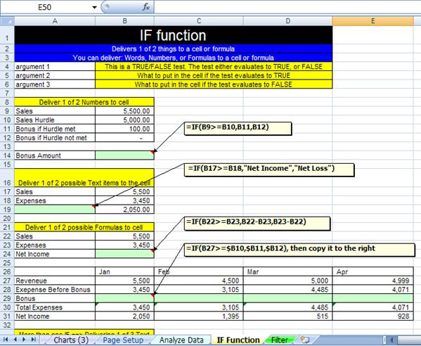
Figure 363
2. Click in cell B14
and type the beginning few characters of our formula: “=IF(“. In Figure 364 you can see the beginning characters of our
formula in the cell B14 and in the formula bar. You can also see a function
screen tip that gives you a hint of what arguments are required.


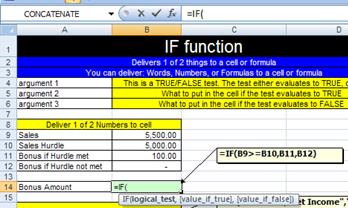
Figure 364
3. Type the logical
test (Figure 365). This logical
test says “If Sales are greater than or equal to the Sales Hurdle”. This logical
test will come out to be TRUE or FALSE.
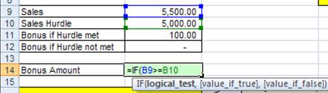
Figure 365
4. Next, we type a
comma. As seen in Figure 366, the screen tip
highlights with bold the next argument that is needed. We can see that we must
tell the IF function what to put in the cell if the logical test comes out to
be TRUE.
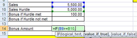
Figure 366
5. As seen in Figure
367, in order to tell the function what value
goes into the cell if the logical test is TRUE, we click on the cell with the
$100 bonus, cell B11.
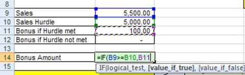
Figure 367
6. As seen in Figure
368, we complete the formula by adding the last
argument and ending parenthesis to our IF function. This last argument tells
the IF function what to put in the cell if the logical test is FALSE.
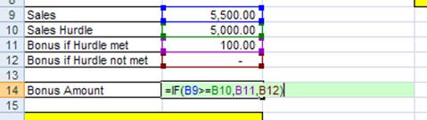
Figure 368
7. Hit control +
Enter to enter our formula into the cell. As seen in Figure 369, the IF function delivers the $100 bonus to the
cell because our Sales number, $5,500, is above the Sales Hurdle number,
$5,000. But what if our mean boss changed the Sales Hurdle number to $6,000?
What would happen to our $100 Bonus?
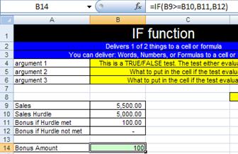
Figure 369
8. To see the IF
function in action, pretend you are the mean boss and change the Sales Hurdle value
in cell B10 to the value $6,000 (which is above your Sales number. As seen in Figure
370, the IF function looked at the logical test
Sales>=$6,000 ($5,5000>=$6,000), came to a FALSE conclusion, and then put
the $0 amount in cell B14.
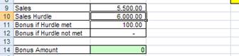
Figure 370
9. Now change your
Sales number to $6,000. As seen in Figure 371,
because the logical test Sales>=$6,000 ($6,000>=$6,000) was TRUE, the
TRUE amount of $100 was put into cell B14.
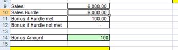
Figure 371
10. Before you try the
remaining IF functions on your own, let’s look at the completed IF function
formula in cell A19 in our formula bar in Figure 372.
Here we can see that the logical test is whether or not Sales are greater than
Expenses (Sales>=Expenses), if this is TRUE, we want out label to read “Net
Income”, otherwise if it is FALSE, we want our label to read “Net Loss”.
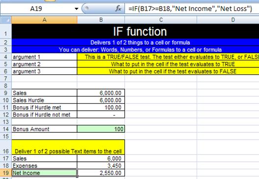
Figure 372
11. In Figure 373 , we can see that if we were to change or Expenses
to be $7,000, the labels updates because the IF function formula puts the words
“Net Loss” in the cell because the logical test evaluates to FALSE.
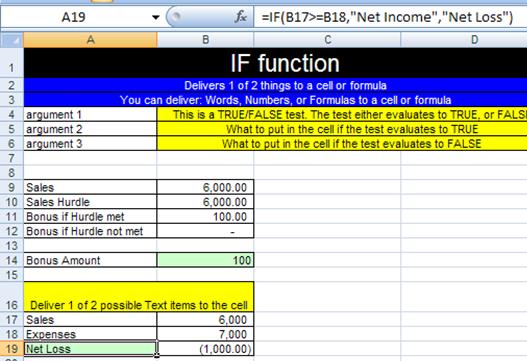
Figure 373
This is just the beginning of what Excel can do for you. We
have looked at the following topics:
1.
What Is
Excel?
2.
Rows,
Columns, Cells, Range Of Cells
3.
Worksheet,
Sheet Tab, Workbook
4.
Save As
is different than Save
5.
Ribbons
6.
Quick
Access Toolbar (QAT)
7.
Scroll
Bars and Selecting Cells
8.
Keyboard
Shortcuts and the Alt Key
9.
Two
Magic Characters In Excel
10.
Math
11.
Formulas
12.
Functions
13.
Cell
References
14.
Assumption
Tables/Sheets
15.
Cell
Formatting
16.
Charts
17.
Page
Setup
18.
Analyze
Data: Sort, Filter, Subtotals, PivotTables
19.
IF
function
The key to learning Excel is to learn the theory of how to
create Excel spreadsheets so that you can accomplish your tasks quickly and so
that everything is updateable later. Inevitably, when we create a spreadsheet,
later when we use the spreadsheet again, we need to change it to accommodate
some new parameter that we had not initially considered. If you follow theses Efficient
Spreadsheet Construction Guidelines, your setup, usage and edit time
can be reduced significantly. In addition, you will have more fun with your
job. Still further, you will become the Excel-master at your job and others
will look to you for guidance! This is great because in this world of
“Excel-Is-The-Default-Program-That-Everyone-Uses-Every-Day”, you will get
promoted more quickly and have more time for vacations! Plus, this Excel stuff
is just plain FUN!!
Efficient Spreadsheet Construction
Guidelines:
Rule
# 1: Learn Excel well so you can have fun working efficiently, gain promotions
quickly, and have more vacation time. 4
Rule
# 2 = Always name your worksheets so that you can identify amongst the various
worksheets. 8
Rule
# 3 = Always name your workbook and save it to a location that you will be able
to find later 9
Rule
# 4 = Learn keyboard shortcuts in order to save time. 31
Rule
# 5 = When the equal sign is placed as the first character in a cell that has not
been pre-formatted as Text, it tells Excel to create a formula. 33
Rule
# 6 = Do not type data that can vary into a formula. Instead place the data in
a cell and refer to it using a cell reference. (A tax rate is a good example of
a number that can vary; 12 months in a year is an example of data that will not
change). 34
Rule
#7 = Use “Enter”, “Ctrl + Enter”, “Shift + Enter”, or “Tab” to enter a formula
into a cell. 37
Rule
#8 = We must learn the symbols that Excel uses for math and we must know the
order of operations. 38
Rule
#9 = By typing the numbers that can vary into cells and referring to them in
our formulas using cell references, we gain the ability to edit formulas easily
and check different scenarios without much effort. 45
Rule
#10 = Using Excel’s built in Functions can simplify and shorten formula
creation. 51
Rule
#11 = Finding functions in Excel can be accomplished by reading the
descriptions, searching for a common sense name in the list of functions, or by
using the “Search” feature in the Insert Functions dialog box. (You can search
Google or the mrexcel.com site also.) 51
Rule
#12 = Figuring out what arguments to use for a given function can be
accomplished by reading the descriptions, or by clicking the help button in the
Argument dialog box. 51
Rule
#13 = Using functions with ranges instead of a collection of individual cells
allows structural updating to spreadsheets more easily. 54
Example
of Rule #13: Use “=SUM(A13:A17)” instead of “= A13+A14+A15+A16+A17”. 54
Rule
# 14 = Use of relative, absolute and mixed cell references reduces spreadsheet
setup time, allows quick updating to setup structure, and will allow us to use
many of Excel’s advanced features and tricks. 67
Rule
# 15 = When you use the fill handle to copy a formula across the rows and then
across the columns, it is a two-step process. First copy it down, then let go
of mouse, then copy it over (or visa-versa) 67
Rule
# 16 When you copy a formula that has a relative cell reference component, the
relative cell reference changes relatively. When you cut a formula with
relative cell references component, the relative cell reference does not
change. 69
Rule
#17: All data that can vary goes into a properly orientated assumption table
that is at least one blank row/column away from the main table (it can also be
placed on an entirely separate sheet). An example of data that can vary is a
tax rate. An example of that data that will not vary is 12 months in a year.
Although a properly orientated assumption table is not always possible, the
idea is to have the labels in the table orientated (horizontally or vertically)
in the same way as the assumption table If we do this, editing formulas,
what-if analysis and formula creation is dramatically more efficient than if we
do not utilize assumption tables. 80
Rule
#18: Properly orientated assumption tables allow for mixed cell use and results
in reduced time creating formulas. 80
Rule
#19: Cell Formatting is the façade that sits on top of data and formulas. What
you see is not always what sits in the cell. 89
Rule
#20: Because formatting (such as currency) is like a façade that sits on top of
the number, when you have a formula that has the potential to yield more
decimal places than the format displays, use the ROUND function. 97
Rule
#21: With Date number format, Excel sees the number of days since. 100
Rule
#22: With Time number format, Excel sees the proportion of one 24 hour day.
This allows us to make time math calculations. 104
Rule
#24: Before you use Excel’s Data Analysis Tools: the data must be in proper
Excel “List” or “Table” Format. This format is as follows: 1) First row has
field names with formatting that is different from the rest of the data; 2) No
blank field names; 3) Columns are called Fields; 4) Rows are called records; 5)
No blank columns (fields); 6) No blank rows (records); 7) Blank rows and
columns and/or Excel’s column headers (A, B…) and/or row headers (1, 2…) must
separate the Excel List from other data. 121
Rule
#25: Before click the “A è Z” icon button in the Sort & Filter Group on the
Data Ribbon, make sure your block of data is in the Proper Excel List/Table
Format and highlight only one cell in the field you want to sort. 124
Rule
#26: Using the Sorting or Filtering features in Excel can save a tremendous
amount of time as compared to accomplishing the same sorting or filtering tasks
manually. 126
Rule
#27: Before adding automatic Subtotals, sort your field. If you want to add a
Subtotal to a Subtotal, Be sure to uncheck the. 129
Rule
#28: When your data is in Proper Excel List Format, PivotTables are the most
powerful tool in Excel. Don’t be afraid of them, there are just tables with
variables on the left (Row) and top (Column) side and an intersecting
calculation in the middle (such as summing)! 134
Keyboard shortcuts
Excel Options Area (Keyboard Shortcut Alt F + I)
Ctrl + F1 (This is a toggle that will hide and unhide the Ribbons)
Save As (Keyboard Shortcut = F12)
Save = Ctrl + S
Spelling = F7
Undo = Ctrl + Z
Copy = Ctrl + C
Cut = Ctrl + X
Paste = Ctrl + V
Go to cell A1 = Ctrl + Home
Select two cells and everything in-between = Click on first cell, hold
Shift, Click on last cell
Select cell ranges that are not next to each other = click on cell or range
of cells, Hold Ctrl, click on any number of other cells or range of cells
Ctrl + arrow key = move to end of range of data, or to beginning of next
range of data
Method of placing cell references in formula after you have placed an equal
sign as the first character in the cell: 1) use mouse to click on cell, 2) use
arrow keys to move to cell reference location
Keyboard shortcut: Shift + F3 = open Insert Function dialog box
Cancel the formula in the middle of
creating it (Shortcut key = Esc)
Formula is entered in the cell and
the cell is selected (Shortcut key = hold Ctrl then tap Enter)
Ctrl + Page Up è
moves you up through the sheets
Ctrl + Page Down moves you down
through the sheets
Keyboard shortcut for the SUM
function is Alt + “=”
Keyboard shortcut for Range Finder
= F2
Keyboard shortcut F4 key: Toggles
between the four types of cell references
Keyboard shortcut Insert Row = Alt + I + R
Delete key = delete cell content
but not format
If you have a range highlighted and
you place a formula into the white cell, when you hold Ctrl and tap Enter, the
formula is placed into all the cells that are highlighted
Tap Alt, then tap I and then tap C
(Alt + I + C is the keyboard shortcut for Insert Column)
Hold Ctrl, then tap the “*” key on
the number pad (this selects the table)
Ctrl + 1 opens the Format Cells
dialog box
Hold Ctrl and tap ; (semi colon) to
put Today’s date in the cell
To bring the format back to the
“General format, Hold Ctrl and Shift and tap ~
Hold Ctrl and Shift and tap the $
key (this is the keyboard shortcut for the Currency format)
Hold Ctrl and tap the “A” key
(keyboard shortcut for Select All)
Hold Ctrl and Click on the Chart
(This selects the chart so that you can move it).
Keyboard shortcut for the Formatting
Chart Element dialog box =: Ctrl + 1
Keyboard shortcut for Page Setup:
Alt + P + S + P (Tap each key in succession)
(Keyboard shortcut for Headers and
Footers is Alt + N + H (this puts you into Page Layout View with the Headers
enacted), and the keyboard shortcut to get out of Page Layout View is Alt W + L
(this puts you back in Normal View)
Keyboard shortcut for Filter: hold
Ctrl and Shift, then tap the “L” key
Open the Subtotals dialog box with
the keyboard shortcut: Alt + A + B