216 Amortization Project
Amortized loan:
i. An
amortized loan is a loan that requires interest payments to be made
periodically. The period is typically one month for a home loan. When an
individual makes the monthly payment, part of the payment is interest and part
of the payment is a reduction in the loan amount.
Interest:
ii. Interest
is like rent on money
iii. If
the borrower agrees to pay an annual interest rate of 12%, the monthly interest
rate would be 6%/12months = .5% per month.
iv. If
the current monthly balance of the loan is $250,000, the interest calculation =
*
$250,000*.5% = $1,250
v. If
your monthly payment sent to the banker (creditor) = $1,348.99, then the two
parts are:
*
$1,250 = Interest paid to Banker
*
$1,348.99 - $1,250 = $223.99 left over to reduce
your current loan balance
vi. After
the banker received your payment of $1,348.99, your current balance for your loan
would =
*
$250,000 - $223.99= $224,776.01
Amortization tables:
i. An
amortization table shows what part of a monthly loan payment (PMT) goes into
the banker’s pocket as interest and what part is applied to the principal loan
amount (Current Balance of Loan) for every payment.
Directions
for creating the 216 Amortization
Project
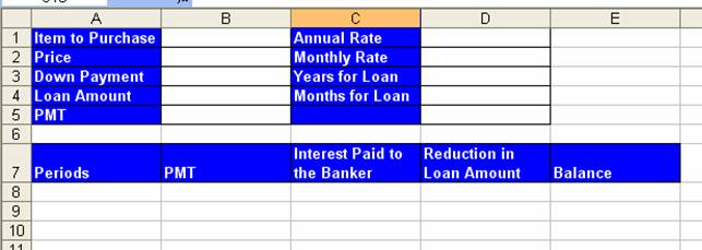
1)
Looking at the picture below, type the text, add color
to the cells and text, add borders, add word wrap to row 7, and resize the
columns so that the text is easy to read
2)
Name the sheet tab “Bank Loan for House (1)”
3)
Save the workbook with the name: “Amortization Table”
4)
Add the following page set up elements:
i. Margins
Tab: center on the page horizontally
ii. Header/Footer
Tab:
*
Custom header:
i.
Left section: file name
ii. Center
section: sheet tab name
iii. Right
section: date
*
Custom footer:
i.
Center section: “Page 1 of ?”
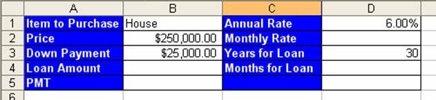
5)
Add the following data:
6)
In cell A8 type the number 0
7)
Create a formula in cell A9 that is “one above plus 1”
8)
Copy the formula in A9 to the range A9:A368
9)
Highlight the range A7:E368 and then click the “All
Borders” button on the Formatting Toolbar
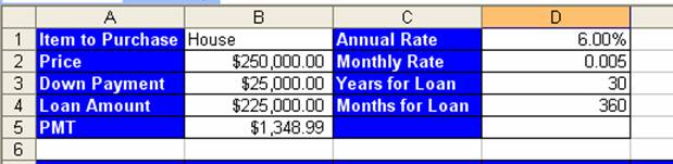
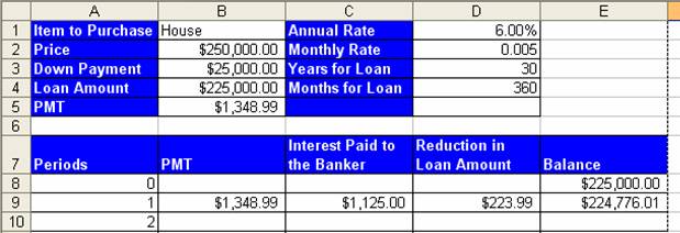
10) Create
the appropriate formulas in cells B4, B5, D2, D4 so that the assumption table
looks like this:
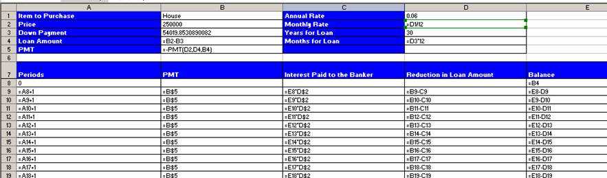
11) Create
the Appropriate formulas (with mixed cell references) in the cells E8, B9, C9,
D9, E9 so that the zero period and first period lines look like this:
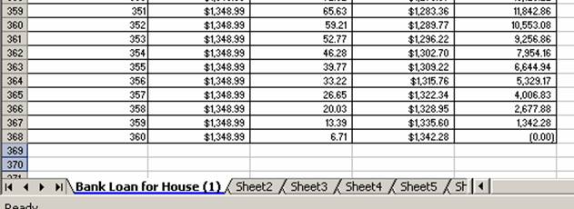
12) Copy
the formulas in cells B9, C9, D9, E9 down to row 368 by highlighting the range,
pointing to the fill handle, and double clicking the fill handle with the
“angry rabbit”
13) Look
at the bottom of the table to verify that the formulas are correct. Then fix
the apparent “negative zero.”
14) Wow!
Finance is Fun!